Testing Difference of Means in Two Independent Samples (Equal Variances Assuming) | BIO733_Topic136

Duration: 7:58 1171 transcript words EN summary

Video summary

This module focuses on conducting a hypothesis test for the difference between means in two independent samples, specifically under the condition that population variances are unknown and assumed to be unequal. The primary objective is to determine whether the mean of the first group differs significantly from the mean of the second group. Before performing calculations, it is essential to verify that the samples are independent and randomly drawn, and that the populations follow a normal distribution. In this specific scenario, since the variances are not assumed to be equal, the analysis utilizes separate variance estimates rather than pooling them, which distinguishes it from cases where equal variances are assumed. 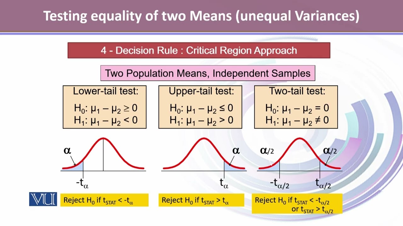The hypothesis testing framework allows for three types of alternative hypotheses: lower-tail, upper-tail, and two-tailed tests, each defining different conditions under which the null hypothesis is rejected. For a two-tailed test with a significance level of alpha equals 0.05, the decision rule involves comparing the computed test statistic against critical values derived from a modified t-distribution that accounts for unequal variances. The test statistic is calculated by dividing the difference between sample means by the square root of the sum of the variance-to-sample-size ratios for both groups. If the absolute value of the computed statistic exceeds the critical threshold, the null hypothesis is rejected, indicating a statistically significant difference between the population means. To illustrate these concepts, the video presents an example involving a study on aortic stiffness index in patients with hypertension compared to healthy control subjects. The data shows that the hypertension group had a mean stiffness of 19.16 with a standard deviation of 5.29 based on 15 participants, while the control group had a mean of 9.53 with a standard deviation of 2.69 from 30 participants. After confirming that the samples are independent and assuming normality, the researcher calculates the necessary weights for each group to determine the critical values using a t-distribution table. The resulting computed test statistic is found to be 6.63, which is substantially larger than the calculated critical value of approximately 2.133. Based on these calculations, the conclusion is that the null hypothesis is rejected because the computed test statistic falls into the rejection region. This leads to the final determination that there is a significant difference in the mean aortic stiffness index between the two populations. The analysis demonstrates that individuals with hypertension exhibit much higher aortic stiffness compared to healthy controls, supporting the researchers' interest in reducing this metric. While the example uses the critical region approach, the transcript notes that the same conclusion can be reached using the p-value method, where the null hypothesis would be rejected if the p-value were less than or equal to the chosen significance level of 0.05.

Read the full video transcript

This module talks about testing difference of means in two independent samples assuming that the population variances are unknown and they are unequal. So here the goal for the testing hypothesis for the difference between two population means is to find out that whether the mean for the first group is equal or not equals to the mean for the second group. The very first thing we need to figure out is that whether the population means uh the populations are independent or not. So as uh the different data sources may arise they can be dependent which is also called related or paired against a situation where are both the samples can be independent where the sample selected from one population has no effect on the sample selected from the other. We can think of two possible cases where the standard deviations or the variances are unknown but they are assumed to be equal. We use pooled variance t-test and we use SP as the estimate for unknown sigma. On the other hand when sigma one and sigma two are unknown but they are not assumed to be equal we calculate S1 and S2 as estimates for the unknown sigma one and sigma two and use a separate variance t-test. Here in this scenario we are considering the second option where sigma one and sigma two are unknown and they are not assumed to be equal. Hypothesis can be stated in three possible ways where we can state it as a lower tail test when the differences between two mean is less than zero as an alternative hypothesis or it could be upper tail test where difference between two means is greater than zero. Can be stated as alternative hypothesis, and thirdly, it can be stated as as a two-tailed test where the difference is not equals to zero as an alternative hypothesis. We will contain the usual level of significance that alpha equals to 0.05. Then, uh we're going to check for the assumptions. The first assumption states that samples are randomly and independently drawn. The second assumption states that population are normally distributed. And the third assumption states that population variances are unknown, but they are assumed to be unequal. So, when in the case when population variances are equal, but they are drawn from normally distributed populations, the test statistics for testing H0 that mean mean of the first group is equals to the mean of second group is denoted by T prime, which is the estimate of the difference in the means, that is X1 bar - X2 bar μ1 - μ2 / S1 squared over N1 + S2 squared N2. But here, the critical value of T prime for an alpha level of significance and a two-sided test is approximately uh you know, T distributed with T prime 1 - alpha / 2 is W1 T1 + W2 T2 / W1 + W2. Then, uh we make this uh decision rule. And here we are using the critical region approach. Then, if it's a lower tail test, we reject H0 if T statistics, which is T computed, is less than - T alpha. If it's upper tail test with a greater sign in the alternative hypothesis, we reject H0 if T computed is greater than T alpha. But if it's a two-tailed test, we reject H0 if T stat is less than - T alpha by 2 or T stat is greater than T alpha by 2. We can use the usual P value approach to make our decision rule as well. Here we reject H naught if P value is less than equals to alpha. Then we'll cal- we'll make some calculations and give our conclusion. Let's take an example. The researcher wanted to examine the subjects with hypertension and healthy control subjects. One of the variables of interest was the aortic stiffness index. Measures of this variable were calculated from the aortic diameter evaluated by M-mode echo- echocardiography and blood pressure measured by sphygmomanometer. Generally, physicians wish to reduce aortic stiffness in the 15 patients with hypertension, which we are taking it as a group one. The mean aortic stiffness index was 19.16 with a standard deviation of 5.29. Whereas in the 30 control subjects, it's treated as a second group. The mean aortic stiffness index was 9.53 with a standard deviation of 2.69. So we wish to determine if the two population represented by these samples differ with respect to mean aortic stiffness index. We state our data that we know that sample size for the group one is 15 and sample size for the group two is 30 with their respective means X1 bar for the group one and X2 bar for the group two is respectively 19.16 and 9.53 with their standard deviations for the group one is 5.29 and standard deviation for the group two is 2.69. It's very important that we test for the assumption. Since the data constitute two independent random sample, independent assumption is fulfilled and one from a population of subjects with hypertension and other from a control group. And we assume that aortic stiffness values are approximately normally distributed. And if we ever have to test, we can use Kolmogorov-Smirnov test, or we can use Shapiro-Wilk test to test for the significance of the normality in both populations. And lastly, the population variances are unknown, and they are assumed to be unequal. We state our null hypothesis, mu1 minus mu2 is equals to zero against alternative that both the means are not equal. So, the test statistics is given by the equation given on the right, where T prime is X1 bar minus X bar 2 minus mu1 minus mu2 divided by S1 squared over N1 plus 2 squared over N2. And the distribution of the test statistic is given by uh the equation we have stated on the right does not follow the student T distribution. We therefore obtain its critical values by equation, and our decision rule states that that at alpha 0.05 before computing T prime, we calculate W1, which is standard deviation squared of divided by the size of the group one. It is 1.8656, and W2 is the standard deviation squared divided by the uh number of observation in the group two, which is 0.2412. So, uh using the table of the T distribution, we find that T1 and T2 are 2.1448 and 2 T2 as 2.0452. So, using these values, our statistics turn out to be 2.133. So, our decision rule then is to reject H0 if computed T is either greater than equals 2.133 or less than 2. 1 minus 2.133. So, we computed this T statistic. Our value turned out to be 6.63, and the statistical decision states that that since 6.63 is greater than 2.133 we reject our null hypothesis and conclude that on the basis of the results that the two means are different. One can also use the P-value approach for this test.