Testing Difference of Means in Two Dependent Samples (I) | Applied Biostatistics | BIO733_Topic140

Many times when we are carrying out some experiments and we are interested in looking at the effect but we cannot obtain independent observations from two different samples. This is a situation where we get our data coming from related samples or maybe one respondent giving two information. This is a situation where our samples are dependent. And this specific situation is called paired samples or the samples with multiple responses. In this module we'll learn that how to perform the appropriate test when we have two samples which are dependent. Let's first talk about paired comparisons. It's a method that's frequently employed for assessing the effectiveness of a treatment or experimental procedure. One that makes use of related observations resulting from non-independent samples. And a hypothesis that's based on this type of data is known as paired comparison test. It's not always possible to obtain sample that is independent. Hence there are certain reasons for pairing the data. So it frequently happens when the true differences do not exist between two populations with respect to the variable of interest but presence of extraneous sources of variation may cause rejection of the null hypothesis. In such instances true differences may be masked by the presence of extraneous factors that are pre-present or they have been there because of the process we are using. So, the objective in paired comparison test is to eliminate a maximum number of sources of extraneous variation that masks the real effect. So, that we can establish that whether there is a true difference between the groups or not. Pairing is a process that we often use to make sure that our two groups are matched. They are matched on a number of ways. The first is when the same subject may be measured before and after receiving some treatment. The other scenario is when littermates of the same sex may be assigned randomly to receive either a treatment or a placebo. Or their pairs of twins or siblings may be assigned randomly to two treatments in such a way that the members of a single pair receive different treatment. Or when we are comparing two methods of analysis the material to be analyzed may be divided equally so that one half is analyzed by one method and other half by another method. Or one is doing some matching of individuals on certain characteristics. For example, digital dexterity which is so which is closely related to the measurement of interest. Say post treatment scores or some test requiring digital manipulation. When we have the paired data, we resort to test them using paired sample tests. And when we are performing paired sample tests instead of performing the analysis with individual observation, we use DI where DI is the difference between pairs of observations. The choice of using either parametric test or non-parametric test for the comparison of dependent sample solely depends upon the fulfillment of certain assumptions. And if those assumptions holds true we prefer parametric test which is paired samples t-test. But if the assumptions are not met then it's non-parametric counterpart is used which is known as Wilcoxon signed rank test. Here are some assumptions that we need to test when we are making comparison between paired groups. The very first assumption asks for our variables of interest to be continuous. They can either be measured on a ratio scale or an interval scale. The second important assumption is independence. Though we are talking about dependent samples but still we are looking for independence but this independence does not mean the independent samples but it is the independence that the observations within the sample are independent to one another. Third important assumption is that of normality where we test the differences of the pairs and believe that that follows the approximately normal distribution. And the fourth important assumption is that there should be no outliers in the data. So if there are any extreme values in the data then we can go with the appropriate test. So when we test these assumptions and all these assumptions holds true we can conclude that we can use parametric test. And when we are using parametric test for the comparison of difference between two means in the dependent samples, we perform a test that's called paired samples t-test. In a paired sample t-test, if you look at the process of testing of hypothesis in paired sample t-test, the very first thing is to state the null hypothesis and alternative hypothesis. The null hypothesis is stated as mu d equals to zero against alternative that mu d is not equals to zero. Here, mu d is the difference between the means of the two groups. The second step requires us to state the level of significance, which is alpha is equals to 0.05. And thirdly, the test statistics. And since we say all the assumptions hold true, >> [snorts] >> we will perform paired samples t-test where t test statistics is defined as d bar minus mu d divided by standard deviation s d bar. Here, d bar is sample mean of difference where mu d is hypothesized population mean difference. And s d bar is the standard error for the difference, which is s d divided by under root n. Where s d is a standard deviation of the sample differences. And as a fourth step, we perform certain calculations. Here, we'll perform them manually as well as using SPSS. And then, decision rule. We reject h naught if p value is less than equals to zero. Or we can use critical region approach using usual t statistics and t distribution. And finally, we state the conclusion. And our conclusion can be uh needs to be statistical conclusion and application conclusion. Let's take an example where we have a data that was obtained from Gorton John M. Morton et al. examined gallbladder function before and after fundoplication. This is a surgery that's is to stop stomach contents from flowing back into esophagus. In patients with gastro- esophageal reflux disease, the authors measure gallbladder functionality by calculating the gallbladder ejection fraction, which is measured as percent. So, we wish to know if these data provide sufficient evidence to allow us to conclude that fundoplication increases GBEF functioning. So, here we have the data given in percents before and after the treatment. Before the treatment values are stated as pre-op. That's a prior to operation. And then there's post-op. All these values are stated in percentages. So, we want to make comparison between these two. So, here we'll say that sufficient evidence is provided for us to conclude that the fundoplication is effective if we can reject the null hypothesis that the population mean change, that is mu d, is different from zero in the appropriate direction. Further, we shall perform the statistical analysis on the differences in pre-op and post-op GBEF. We may obtain differences in one of the two ways, whether we can subtract post-op from pre-op or pre-op from post-op. One has to make a choice which one they use out of these two. So, here we have this data from pre-op and post-op and we want to take the differences and in this situation we are taking di, which are the differences, as post-op minus pre-op and the difference differences turn out to be 41.5, 28.2 and likewise for the rest of the other observation. Now, while we are performing paired sample t-test, it's very important that we We for the assumptions. As stated earlier, we have four assumptions to take care of. 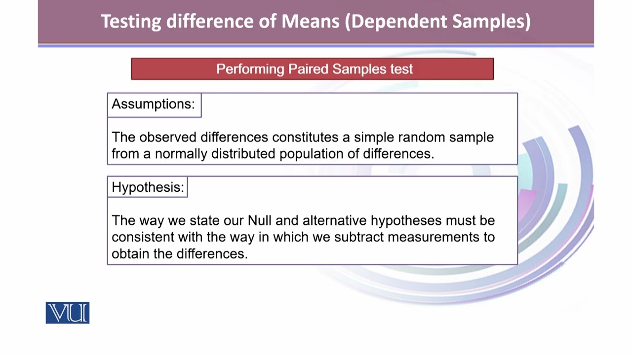But here for the sake of uh So, we assume that the observed differences constitute a simple random sample from a non- normally distributed population of differences. The next step is the hypothesis. The way we state our null hypothesis and alternative hypothesis must be consistent with the way in which we subtract measurements to obtain the differences. So, the question is that what does it mean by calling something effective? So, in the present example, we we want to know if we can conclude that fundoplication is useful in increasing GBEF percentage. So, the question is that what does it mean by calling something to be effective? And especially in the present example, we want to know if we can conclude that fundoplication is useful in increasing gall bladder ejection fraction percentage. We expect the post-op percent to be larger than pre-op percent. Hence, the difference post-op minus pre-op should tend to return positive values. And if we are making the difference from post-op minus pre-op, our hypothesis should be stated in the same way, too. Furthermore, we would expect the mean of population of such differences to be positive, too. Having positive result indicates that the values in the pre-op are smaller as compared to the values in the post-op. And here, the higher percentage indicates that the treatment is effective. So, under these conditions, asking if we can conclude that the fundoplication is effective is the same as asking if we can conclude that the population mean difference is positive, which means that it is greater than zero. So, using this information, our null and alternative hypothesis can be stated as H0 μD is less than equals to zero against the alternative hypothesis that μD is greater than zero. But, if we had obtained the differences by subtracting the post-op percent from the pre-op weights, that is pre-op minus post-op, our hypothesis would have been reverted. And it could have been stated as μD greater than equals to zero against alternative hypothesis that μD is less than zero. Because if we do pre-op minus post-op, then the values have to be negative and post-op percentages should be greater, contrary to the previous hypothesis. But thirdly, if the question had been such that two-sided test was indicated, the hypothesis would have been H0 that μD is equals to zero against alternative hypothesis that μD is not equal to zero. But here, in our situation, since our interest is in looking at if fundoplication is effective, and to do so, we expect that post-op values should be larger. And having the difference from post-op minus pre-op, we expect the positive values, the values which are greater than zero should be there to prove that fundoplication is an effective treatment. Hence, the first hypothesis that says H0 μD is less than equals to zero against alternative hypothesis that μD greater than zero is the most appropriate hypothesis in this situation. So, our hypothesis is stated, our level of significance is assumed to be 0.05, which is 5% chances of making type one error. And after that, we have the test statistics, assuming all the assumptions stated priorly are true, we have paired samples t-test with t statistics is d bar minus mu d over s d bar. Using this information and making the calculations, we have 12 observations. We have taken the differences. D bar turned out to be 18.075 against the stand s d squared equals to 1068. Using this information in t statistics are t desert turned out to be 1.9159. It's a decision rule where one can use the p value approach where we can say that we reject h naught if p value is less than equals to alpha, that is 0.05. Or one can use critical region approach where we can assume and let that alpha 0.05 the critical value of t is 1.7959. And we reject h naught if computed t is greater than or equal to the critical value and it's been reflected in the picture given below. And in this figure, the shaded region is uh the rejection region. And the other unshaded region in this bell curve is non-rejection region. And if our test statistics falls in the rejection in the shaded region, that's the rejection region, we will reject our null hypothesis. And if it falls under non-rejection region, then we will not be able to reject our null hypothesis. Using this information, we already know that our test statistics value t calculated is 1.9159, which is greater than 1.7959. Hence, it falls into the rejection region. And once it fall into the rejection region, we may conclude that we reject the null hypothesis and our statistical conclusion clearly states that that we are rejecting the null hypothesis again and our application conclusion will state that we may conclude that fundoplication procedure increases gallbladder ejection fraction functioning.