Statistical Rethinking Lecture B10 - Hidden Markov Models

Uh, welcome back everybody. This is the last lecture of the 2026 um, instantiation of statistical rethinking. Here in the experience section, there I took a poll um, and I got uh, a number of responses from people and the overlap was in more time series modeling. Uh, and one category of that is hidden Markov models. So, that's what I'm going to try to do today. This is going to overlap with some of the uh, previous material in in uh, themes like measurement error and the like. But, there'll be some new mechanics and computational tools I can teach you as well. Uh, remind you uh, of the part of the workflow where we have done most of the action in this course and how it's going to relate to the topic today. On the left you have just the the very left-hand side of this core Bayesian workflow I've been showing you and I augmented it in the last, I don't know, three, four lectures with measurement models. We've been dealing a lot more explicitly with measurement models, not just what nature does, which is the generative model. Right? Nature does stuff whether we observe it or not. Uh, things happen. Uh, then we observe those things through process called measurement and often we ignore that. Right? We teach we treat our measurements as if they were delivered by angels on golden platters or something. But, sometimes and sometimes you can do that. Sometimes you can safely ignore measurement error or just assign a sigma to it or something like that and get away with it. But, often you cannot because there is differential measurement error or um, response biases, uh, patterns in missing uh, data that are related to the measurements themselves. Um, I gave you a really protracted example with censoring, remember? Uh, of an a case where you really cannot ignore the missingness because you will get a systematic bias in an infinite sample. Samp increasing sample size doesn't fix these problems and so we spend time modeling measurement as well. We're going to do that today, too. Um, this is the hidden Markov models uh, state-based models are about measurement um, as as well as about the generative processes. And the the idealized problem we deal with in these latent state and and hidden Markov models is a case where there's some cause of interest X and it's unobservable. It's a latent state. It could be an internal state of an organism. Uh, it could be an institutional configuration. Um, it could be a macroeconomic state. There's all kinds of interesting things like that where the causes of interest are in principle not detect not directly measurable, but they exist. Yeah. Uh, uh, that makes life fun. Uh, there are things that we could in principle observe and these are the Ys. Um, and uh, the X's influence the Ys and the X's influence one another through time. Um, the Ys are influenced by the X and they can influence one another. Uh, so I'm going to give you examples uh, subject matter examples of this as we go forward. I just want to get the abstraction across to you now. Um, and then there's measurement on top of this cuz it very often we can't observe the Ys, either. Right? We can only get proxies of them. The um, links hair differential equation example, was that the previous lecture? Yeah, the last one we did. That's an example of this in continuous time. Uh, we don't know how many links and hair there are in the in Canada. Right? Nobody does. What we do know is how many pelts were reported. Right? And so that's that's the Y stars up top. But, I hope I convinced you that with some strong and biologically reasonable assumptions, you can infer uh, Ys and X's um, uh, from imperfect measurements like Y stars in many cases. And these things are in principle all examples of what we're going to call hidden Markov models. I'm going to work up to it, though. Um, I want to divide this lecture in two halves with two examples. Uh, first all these models are called latent state models. The causes of interest are latent states, the X's. Um, and to a first order approximation, the entire universe can be modeled this way. Right? Just about everything can be modeled this way. So, every uh, every model we've done, you could consider it a latent state model of some kind. Um, I want to do two examples to build up the complexity. The first is not a time series uh, and I'm going to use this example to introduce you to modeling latent states without the complexity of dealing with sequences of unobservable latent states, which adds more computational complexity. So, just a just a cross-sectional latent state model in the context of strategic learning, which I know some of you in the in my department work on and uh, so this will be this will be useful uh, for for stuff you're working on, I hope. Uh, then I'm going to put a time series and embed the latent state model in a time series. It'll become a genuine hidden Markov model, a very prototypical example. And this is an example I made up and yet it's real. And we will build a Bayesian latent state model of whether the president is dead. Um, okay. So, yeah, work hard for you. I'm I make these new slides all the time. >> [laughter] >> This is um, all right. So, the first one, this uh, uh, this example is a reanalysis of a published data set from this 2018 paper, uh, citation on the bottom. 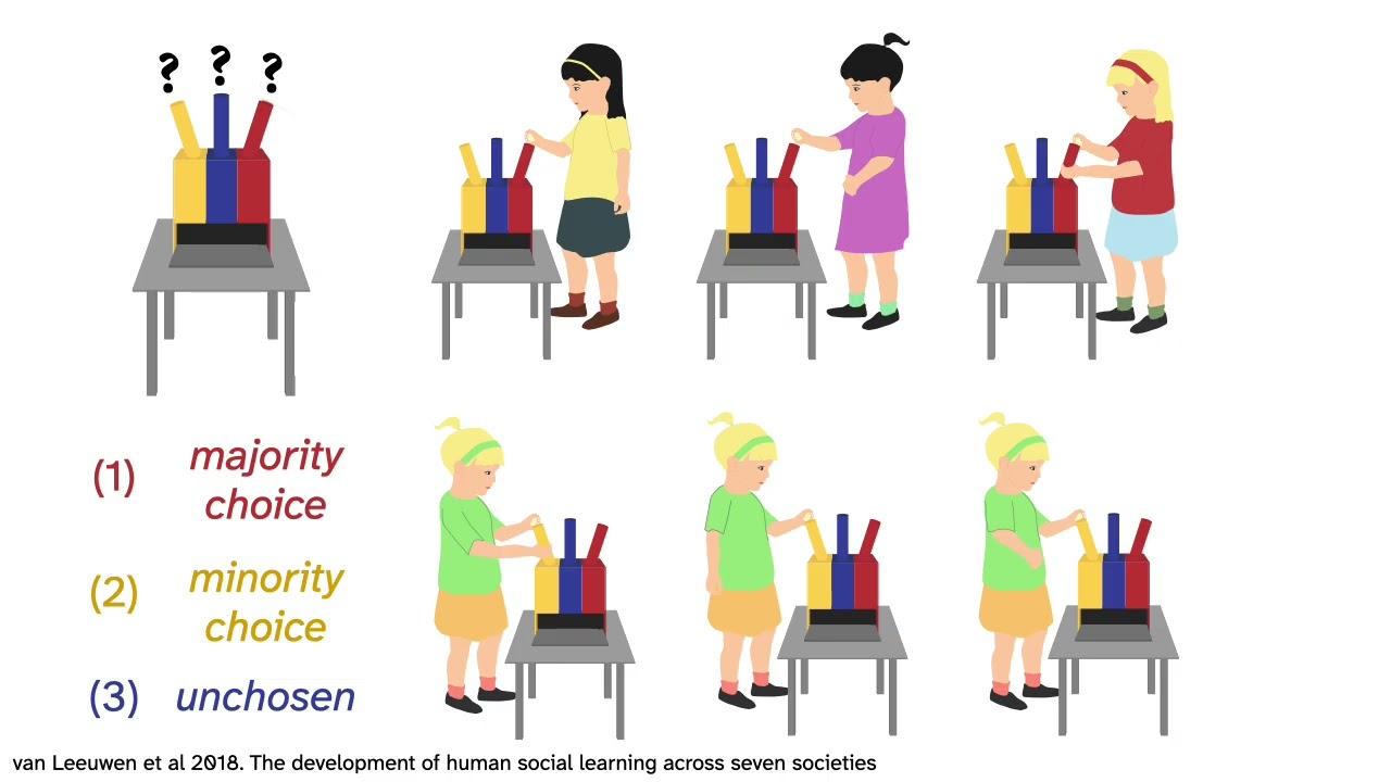Um, this is a child development experiment where children interacted with um, a constructed box which looks something like this. This is an image from the paper of of their drawing of what the box is. Children were given a ball and they would come up and put the ball in one of the tubes. They pick one of the colors and put the ball in the tube and then the box would dispense a toy. And the uh, choice thing give the choice given to the the uh, uh, the children was after they see other children put uh, balls in the different colors, which color did they choose? So, it's a social learning experiment. And in particular, this is, you know, these are developmental psychologists, so everything's counterbalanced in all kinds of ways. Um, uh, the main kind of treatment is to say uh, there are um, each each participant child is going to observe four other children interact with the box before they make their own choice. And so at the top are the first three and each of them chooses the same color. The color is different in different trials and this is what's called the majority choice. So, in this example, it's red. Right? So, three kids choose red. Maybe not all following one another, right? But, um, and then there's a third uh, child. This is the child at the bottom who chooses three times a different color. Uh, why three times? Because you want to be able to say whether the the fourth child, who's the the choice that we're trying to model, is influenced by number of demonstrations. So, the the red is chosen three times and the the yellow is chosen three times here, but one's a majority of children. Right? But, each of them has been chosen the same number of times. Does that make sense? You're trying to distinguish between choice choice uh, heuristics. Um, and then blue, poor sad blue is unchosen. And and now the fourth child is free to choose any of the three. Uh, and they did choose. Uh, [laughter] all of all of the others were chosen by some kids. About 600 kids participated in this uh, at seven different places. Um, and they're in the paper they analyze it by age and location and a bunch of stuff. I just want to focus on what's the relationship between choice patterns and the strategies. The the the motivation for this experiment is do children copy the majority? Uh, if so, how does it develop across age? Uh, and does that pattern vary by culture? The problem is you can't see strategy. It's a question about strategy. The estimate is how are children choosing? Do they follow the majority? Right? Do they follow the minority? Are they simply choosing a color at random? Right? There's a bunch of things they could be doing, but you can't observe that and the experiment is not designed to reveal that in any transparent way. There's an X here. Uh, and what we observe is a Y. The the estimate's about the X's. Does that make sense? I'm going to model this up, though, explicitly. Um, but the basic inferential problem and this is common of all research, it's not unique to this study by any means. I've done research on social learning myself. It's all we always have this problem. The thing you want to estimate is not directly revealed by choices, but it is a function of choices. And and different learning strategies can produce the same choices at different rates in the same treatment. Yeah? Um, so those of us who who do empirical game theory, uh, like I used to, maybe I I will once again, uh, this is the basic inferential problem we deal with when we do uh, game theory experiments. And this this is a game theoretic experiment. So, the basic problem clear? Yeah? Um, in the paper, they uh, ignore this problem. Fortunately, which is why I decided to reanalyze it. So, what did they do? They just used the the color that was chosen um, the color that was chosen by the majority indicates majority pre- preference. And that's the way they do all the analyses. And about two-thirds of kids across all the sites and ages um, chose the majority uh, color in that from their particular trial. Um, and then there's just social information use, which is the sum of majority choice and minority choice. So, or there's the frequency who chose the unchosen color. So, one minus that is taken to be social information use. But, I hope I've convinced you this is not right. Yeah, the these are choices, but they're not strategies. Uh and and the paper conflates the two. So, what would we do instead? Well, we do a latent state model. Uh that's what we do. So, let me show you how that would be done. Well, here's the basic problem. Majority choice is consistent with with many different possible strategies and uh in this uh experiment, I think it's simple enough that there's not a huge range of potential strategies, but nevertheless, I could come up with like five different ones that I'm going to talk about. Um you could choose a random color, in which case a third of the time you make the same choice as the majority. Right? Um you can choose a random demonstrator, and then 3/4 of the time you will choose the same thing, but you're not following majority choice. You're just picking a kid at random cuz you like their bracelet. Right? Something like that. It's what I'd do. Yeah? Nice bracelet. I'm following you. Sort of thing. Um a random demonstration, and then half the time cuz there were there's six demonstrations. And three of them are for the majority choice. Uh so, what could we do instead? Uh this is a case again, I I can't leave the workflow alone for very long. I have to put it in front of you. So, let's come back to the workflow diagram. Um something I haven't emphasized yet in this course, and I wanted to sneak it in at the end out of guilt, uh is the idea that we can use generative models and S demands to think about design as well. In all the examples so far, I've treated data sets like they're delivered to you by by DHL or something. You had nothing to do with them. Yeah, but I that's not how your research goes, right? Yeah? Hopefully, you have some role in planning data collection at least sometimes. There's some looks on faces in the audience. All right. I know some of you do this. This is like 80% of your time is collecting data. Yeah? So, uh we can use these tools also to do design work uh so that we get data sets that have good information on uh uh and match the statistical models as well. And that's what I want to talk about here. It's too late for this experiment, but I'm going to have some We're just going to reanalyze it, but I'm going to have some suggestions as we move forward about what to do. Um First thing we want to do is think about a generative model just to illustrate the point. It's a simple simulation to illustrate what I'm trying to convince you of. So, imagine there's a hundred kids in this simple R script. Um we're going to um say that half of them choose a random color. Uh these are the Y ones. They're just picking a color from one to three. Um that's half of the kids in over two. So, that we're just sampling one of the colors at random, and then half of them the other half follow the majority. And that's what the Y twos are. And the majority color here is two, just in this example, to make it simple. Uh what we observe in this experiment, the Y ones and Y twos are mixed together, and and they cannot be distinguished. And that's what the my lovely bar chart is supposed to illustrate is that the red bar is high, but it's it's composed of unlike things. Right? Different strategies. Uh now, hopefully, this is super clear. Um So, let's consider some other strategies and do this computationally now. Uh we want to infer the unobserved strategy of each child. Um in this case, uh children don't have um I don't think any child was was tested more than once, and so there's really no hope to make an inference about any individual child, but we can make inferences about the proportions of strategies in all the kids. Does that make sense? Um Uh if you wanted to design this for individual kids, you'd need to do you'd need to do repeat observations on individual kids. But there's still information here about the mix of strategies in the population. So, that's where we're going to focus instead. And I'm going to consider a strategy space which just comes from nothing but my feral imagination. Uh you could add your own uh to this, but I don't think these are ridiculous hypotheses. Yeah. None of them involve consulting a horoscope or something like that, right? They're they're things like First one is uh the focus of the paper itself, uh majority choice. They also consider minority choice. There are people uh each of us probably has someone in our friend network who always wants to do uh the opposite of what everyone else is doing. Right? So, this would be the majority choice or uh strategy minority choice or three, which I call maverick. This is the person who says, "Well, no one chose poor blue. I will choose blue." Yeah, we all know that person, too. Yeah. Question. Um do they argue that the point of the minority choice could also be "This girl is onto something. She keeps making the same choice. It's >> understand something." That's not >> thought. Yeah, it's that's that's That would be another heuristic, right? Another way you could choose it, and we need a new another experiment to distinguish that, right? Cuz in this >> that was what they were discussing. No, they're they're just counterbalancing the number of choices, right? Because there was previous research There's the this the paper I'm talking about here, like all papers, is is part of a tradition, and so there previous ones where um the minority choice was just done once, and then the argument was, "Oh, this is confounded with the number of demonstrations, and kids might just be using the number of demonstrations." Like they've seen the color chosen so many times, and that reinforces it. And so, this this experiment was designed to address that, but then that creates another confound. Yeah? So, there's no perfect there's no single experiment which will deal with all that. So, I don't want to uh focus on that too much, but yeah, but that's that could be that could be true in this case, and we can't say if it's different with just have minority color. And if we say there's a a strategy which is choosing uh the color that the fewest number of kids chose, then it would also choose that color, but there's another one which would be um yeah, uh different than that, right? Which is the the fact that that single person has chosen it three times is a better indication of their preference than the individual kids who chose each one once, right? If you're like it's an enthusiasm index or something. Yeah, exactly. Makes total sense. You know? Um Yeah. Good? Yeah? Um fourth is just a random color. Uh the four the you know, the the you have to picture in this experiment, remember there's a participant child who's watching the other uh what you know, a video actually of four kids uh choose, and then they're asked to choose, and they could just be ignoring the video. Right? And then just waiting They're just waiting for you to stop talking, grown-up. Let me put the ball in the box, right? And then they just choose their favorite color. Yeah? Um And I'm going to call that random color, and then the fifth one uh is one that the researchers were concerned about is which color was chosen first. So, these things are counterbalanced. There's a bunch of different videos they recorded. Um and sometimes the um unchosen color comes first, and sometimes the majority color comes first, and sometimes the minority color comes first, but that's coded in the data set, which one came first. And so, it could just be that the kids only pay attention to the first demonstration, and so we want to test for that as well. Okay? Does that make sense? So, you can think of others, and I will show you some code that you can expand. You can add more strategies into this as you like. Okay? Uh I have done experiments in game theory which are like this, but uh have a time series embedded in them, and then the strategy space gets gets even bigger because people have memory, and they can use past choices to do updating, right? And then there's strategic settings, and the strategy space can be fairly big. Good? Yeah? Is that a question, Jeff? Yeah. >> So, I presume this is going to a mixture model, yeah? Like is that what you're saying? It is yes, it is going to a mixture model. That is right. And so, and so Sometimes sometimes in these strategies, what we're trying to estimate is we're trying to estimate population level things, like a marginal rate of substitution. And For example. >> [laughter] >> The economist speaks. And and my big question is My big big question is is like how much power are we losing when you have the initial filter basically choosing the probability that a strategy is chosen, and then you basically lose that additional I presume we lose that additional information that basically feeds into the parameter estimation on in with the in any particular strategy space? Let me I I I think I think this is a good question. Uh and and sorry, the microphone's not picking it up, but we'll come back to this. Um let me present the model structure, and then you can ask it in terms of the parameters labels that I choose, and and then we can make some sense out of it. So, uh this is a categorical model. Um uh each on each trial, there's one choice, and there are three options. So, we've got a three-option categorical model. It's like a Bernoulli choice model, but there's three options now. Yeah? Um And uh theta is a probability vector um that tells you the probability of each choice on trial I. Uh and um the labels I'm choosing here is that label one means the unchosen color, two means the majority color, and three means the minority color. These are behaviors. These are not strategies. Right? That's the whole motivation here. Uh all the action comes into modeling theta. So, uh theta for choice J, where J is one, two, or three, um is going to be uh big angry sigma, right? Which you remember means sum. Right? I'm sorry, this the this typeface, it looks big and angry. It looks really uh you know, it should be nicer looking. It looks very very uh Bauhaus. Uh so, um we're going to sum over strategies S, and there are five strategies in this example. So, we sum over all the strategies, and the first thing in each term in the sum is the prior probability of that strategy. So, this means we're we're averaging. So, this is the mixture model. >> [snorts] >> Yeah? Um times the uh probability of observing that choice conditional on that strategy. So, we don't know the strategy the child used, but we have prior probabilities, and we can computationally make a prediction for each strategy of what a child following that strategy would do in each case. So, we average over them. Why? Because that is the only legal thing to do in probability theory when you're uncertain. Yeah, you have to do this. By the by the axioms. You're The axioms compel you. So, we say in in Bayes' church. Yeah? Uh if you accept the axioms, you must accept this computation. Yeah? But, does it make sense? Uh since we we don't know which strategy there is, but we have priors, the P sub S's. Yeah? I'm going to set them equal across the strategies, but I'll show you that on on the next slide. But, if you had other information, you could weight them differently. And so, once you have prior probabilities, and you can compute the likelihood, that's the big PR Y equals J conditional on S, then you average across. And this is what uh and Jeff asked this with his question, this is what's called a mixture model. Yeah? Does that make sense? Okay. Um And then the last thing is we need prior probability, and so we have this vector P of length five, and uh P is a is a probability, so we want a probability distribution for probabilities. I'll say that again. We want a P is a probability, each element of P is a probability. So, we're going to set a prior on it. So, the distribution needs to be a probability distribution for probabilities. Yeah? So, it's Those of you remember exhibit from MTV's Pimp My Ride, it's like, "Yo dog, I heard you like probabilities." I put probabilities in your probabilities. No. No, what that's the '90s. Um okay. No, so in this case, there's a very good choice um uh the the Dirichlet distribution, which is the um multi-dimensional higher-dimensional uh generalization of the beta distribution, right? You may know the beta distribution probability distribution for a single probability. Uh uh the Dirichlet is the generalization of that, or you might say that the beta is the special case of the Dirichlet for one dimension. Yeah? Um and like the beta, it uh the the Dirichlet is parameterized by pseudo successes, right? This vector of counts, which are the number of prior successes for each one, or observations for each one. That's the same way the beta is parameterized. The alpha and beta the the alpha and beta parameters in the beta distribution are pseudo heads, or whatever you're counting, heads and tails. They're the the prior outcomes of each category. So, here I set it to four each, which is low amounts of evidence that all of them happen. If you made those counts really big, like 100 each, that would be a prior probability that they're all really the same. Uh this is weak evidence that they're all existing, but it doesn't say they're all the same with any confidence because the counts are low. Uh there's a a discussion of this in the book in um I think the ordered categories, it showed the Dirichlet shows up in the book when I teach ordered predictors, and I think there's a bunch of stuff about how they work and some examples in in that chapter, if you want to look and see. Um but, sorry I didn't have time to put it in this lecture. I I There's just not enough time to do it in an hour with all of that. Um Okay, good? Yeah? We're happy? There's some There's some mildly pleased faces in the audience. Yes? Is this good? Um all right, let's look at some Stan code. All right. Uh I think if I really wanted to, I could do this in Ulam. Um but, it's the last lecture, so let's do some raw Stan. Yeah, and for these models, you're going to be so much happier if you just work in raw Stan, or PyMC, or Julia, or whatever, uh because you've just got so much more freedom to just directly express the log probability, and and not fight with abbreviated formula interfaces. Um so, let's do that. So, just keeping the mathematical formula on the right to remind you what it is, um I'm going to walk you through some of the aspects of this code, not all of it. Uh you don't have to be a Stan pro to to see what the relevant issues are here. Um you know Stan has these blocks. At the top, we declare observed variables called data. Then, we declare unobserved variables called parameters. And then, we have this big chunk of code called model, which just computes the log probability of all the observed variables. Yeah? Um So, the first thing to say, we've got this Y's at the top. Um just a vector of observations uh for all from all the trials. And remember, Y can take the value one, two, or three. Um P is uh a vector of probabilities. The There's a special data type called a simplex for this. A simplex is a vector that sums to one. All right, cuz these are prob- the whole They're probabilities of the strategies, right? So, that's what we want to get. We're going to do inference on this simplex for the population of kids who did the experiment. So, we're going to have a prior on P, but it's going to get updated by the choices. We're not going to be able to say what any particular child did um with certainty. Although, there is information about that. You could You could compute it post sampling, right? There's certainly strategies that can be eliminated for a particular child. Yeah? Um but, we what we're in the target of inference here in the simplex is the mixture in the population. Which is not useless. Yeah? Um let's look at the calculations now. Um at the very top of the model block, I declare vector of length five for theta J. This is just a little working variable that lets me uh compute um the elements of theta J that are there on the right, right? Cuz we're going to sum over them. And here's the uh Dirichlet prior. Um and then here's some very ugly code that does all the hard work. So, this is like a multiple choice model. Uh all that's going on here is we loop over children, one to N. And then, we start building up the elements of theta J, all this stuff on the right uh over there, right? Each of the elements uh each of the terms inside the sum is what we're going to calculate. We've already got the P sub S, but we need these probabilities of Y equals J conditional on S, right? You with me? Yeah? Uh so, we do this for each of them. Uh I just make an empty theta J vector uh full of zeros, and then I say, "If the choice equals um two uh uh we go through each of these things. So, the majority choice, if the choice equals two, then the probability um majority conditional on majority, remember conditioning on the strategy. So, the first line uh then it's uh with probability one, cuz two is coded in the data set as the majority choice in the raw data. Otherwise, it's zero. But, zero is the default in the vector. I've already initialized that at the top. And then, the next one for minority choice, if the observed choice was the minority one, number three, um uh then the minority strategy would would do that 100% of the time, probability equals one. Uh then the maverick strategy, which chooses the unchosen, that was coded as number one here. Um Uh and then, we've got the random color, which is always a third for any choice. Do you see that? Theta sub J four equals one over three. Yeah? With decimals in it, cuz otherwise Stan it coerces it to an integer, and we don't want that. Right? Sorry, math in the computer is not real math. You just have to deal with these these monsters like this. Um And then, the follow first strategy, uh uh similar logic. If they if they chose the first one, then this strategy would do that 100% of the time. Otherwise, uh um it it depends upon whether the first matched uh um I don't know what that code is doing, actually. But, it's the right way to do majority first. It's explained in the book. Sorry, I I I don't remember why it's that way. Um majority first equals one. Yeah? Then, if the the choice is two, oh, it's cuz um what the first one was is either the majority or the minority choice. And this is just picking out which of those it was on this trial. That's what it's doing. It's just the way it's coded. Okay. Um and then, we've got to combine all these. So, we've got each of those terms that's in the sum here. And we need to add them together. So, the first thing we do is we need to multiply each of them by the prior probability. So, this is what happens here. We loop over each strategy S, and we get the log I'm doing this on the log scale, cuz that's the way you want to do it. Um Uh we get the log uh of the prior probability plus the log of the of the probability of the data. Right? Cuz on the log scale, probabilities add rather than multiply. Good so far? So, now we've got the log um probability, or the log of each each side of that sum. And now, we need to add them together, and we use this uh little helper thing called log sum exp, which uh some of you are unfortunately already familiar with. This is Yes, I see pain faces in the audience. Um I'm not going to take the time today to explain this, cuz I have a lot of content. But, I have in a previously recorded lecture a whole bonus section about this from the 2023 lectures. And I I don't remember which course it was. Um uh but, there's a bonus section at the end, which is all about functions like this and why we use them. They're They exist for numerical stability of floating point arithmetic is why they exist. This gives us the log of the sum of a bunch of terms that we exponentiate. So, we put in it a bunch of log probabilities and it's going to return the the log of the sum of their exponents. Which is what we want. Does that make sense? It's just It's log sum exponent. It's honest. It tells you who it is. It tells you what it does. Um it's nice and it's just a numeric You always want to use this when you're constructing probability averages like this in a computer. Otherwise, you can get what's called catastrophic underflow. Which is no fun. Yeah? Okay. I'm happy to talk more about this with with anybody after the lecture, but uh it's very good practice and I wanted to have an example of doing this. Um I had a colleague who once wrote to me because they were literally doing a strategy latent strategy model like this and they did not do this and they couldn't understand why their code wasn't working cuz all their probabilities were zero. And it's because they were doing everything on the raw probability scale and it was a time series with like hundreds of choices. And so, any partic- any sufficiently long time series, the probability will approach zero. Yeah, because any particular data set is highly unlikely in a big probability space. And then floating point arithmetic, you start multiplying tiny numbers together and eventually it rounds to zero. Uh this is the reason we do things on the log scale. So, I rewrote their code. Uh Cody and I rewrote their code actually. Cody's not here, but some of you people will know who Cody is. Cody and I rewrote their code so it works now. So, that's uh why I wanted to tell you this. Now, if you ever find yourself in this situation, use log sum exponent or ask me or Cody. Okay, that's That's your heuristic. Good? All right. Was this a fun tour through Stan code? Did you enjoy the ride? Yes? Isn't it soothing? I was I've been told multiple times that my colleagues like to watch me write Stan code cuz it's like watching your friend play a video game, I've been told. The world's most boring video game. But uh there you have it. Okay, inference happens. Um here are the marginal posterior distributions of the elements of theta uh for majority choice, minority, maverick, random color, and follow the first demonstration. Uh see that um there's uncertainty about each of these, uh but these are a lot lower than the um original. So, focus on the top line, majority, the posterior means around 0.25. Remember, the the raw empirical frequency of majority choice is about 2/3. Right? So, this is substantially less evidence. Uh and for social information use overall as well, much lower choice. This With these kinds of of posterior distributions, um what you miss in this marginal display are the correlations. Uh and and I don't know if there's really a good way to deal with that, but of course, you know me, I made an animation. So, there's an animation of these posterior distributions. So, um here are three uh uh uh at the same time, each of the colors is just different draws from the posterior and then each of them is animating between sequential draws from the posterior to show you the correlations in them. Cuz if some of them go up, then the others have to go down, right? It's a simplex. That's the problem. So, there's always strong posterior correlations uh in in vectors like this. Um color is the most uncertain because it's poss- it's capable of explaining the whole data set by itself. None of the others are. Yeah, all the kids could just be choosing their favorite colors. This cannot be eliminated, but it's not very confident that that's true. It could also be that none of them are and that's why the color one swings around the most. Um majority is uh fairly stable as a as a credible heuristic for some fraction of the kids, but it's it's about 0.25 here is the central area, not 2/3 or or about 0.6 uh instead. Um Of course, these probabilities depend upon how many strategies you consider. Uh so, you you always need some scientific background to decide which ones to to put in here. Does this make some sense? Is this good? And I'm I'm not endorsing animations like this as the ideal way to view this, but it's it's just a It's a very difficult thing when you're doing inference on a simplex uh to think about the the how the the error bars are co-varying across the elements. It's a It's a complicated problem. Okay, let me try to summarize a bit and then move on to the second example. Um So, this is an example of what I would call a state-based model. We have hidden states, which are the hypotheses that are meant to explain the data. Inference about them is possible, at least in the right design. Uh it helps if you consider the inferential problem when doing the design. Uh that was not done in this case, unfortunately, but this I was about to say I don't want to single this paper out, but I already have. It's too late. But No, there are lots of papers that make this mistake, right? And so, that's the reason I I want to have an example of it. Um a better design uh that would be able to distinguish majority influence choice from some of the others, you'd vary the size of the majority. Uh there are experiments that have done that. Yeah. Uh but that would be a way to do it. I'm not sure if kids would be tolerant of more complicated designs, so you have to make You have to make compromises when you do child development studies though. Uh what's the general lesson? Uh what we want are latent states, but uh what we have are emissions and you should not confuse them, but use the measurement model. Write down the measurement model, put it into the into the statistical model. Um So, this sets up the second half in the second example, where we take a latent state model like the previous example and we embed it in a time series. So, now you can imagine you had a series of choices from the same kids. Yeah? You could also imagine that their strategies might change from time to time. Right? Do you always use the same strategy for making choices? Don't answer out loud. But uh probably not. So, uh uh these types of models are called hidden Markov models. Um uh What does that mean? Hidden It just refers to the latent states. In general, latent states could be continuous or discrete. I'm going to use a discrete example because I want to show you the simplest structural example that we can think it through. And also, I've already done a continuous time uh hidden Markov model. That was the links hair model. Was a continuous time uh hidden Markov model. I just didn't tell you. Uh Usually, when you hear hidden Markov model, people are thinking about discrete time, but that's actually There are many examples where it's continuous time. Um uh Markov just means memoryless. Uh it's named after a Russian mathematician, but [laughter] uh Now, this is his name. It just means memoryless, so unfortunately. But um Andrei uh What's his Andrei Markov Markovovich, I think was his name, and did a bunch of important work in probability theory. And um Markov processes, named after him cuz he studied them, are memoryless in the sense that only the current state of the system influences the future dynamics. And when you think about that, that's not a strong assumption. That's just how we study physics. Right? Things that happened in the distant past can only affect the future through the present. That's a Markov assumption. Does that make sense? Should I say that again? Things that happened in the distant past can only affect the future through the present. That's a Markov process. I'm I'm happy with that. In fact, I'm very unhappy with models that violate the Markov assumption, right? If something that happened 100 years ago can't have direct psychic influence on current events. Yeah, so lag models do that. Um I complained about those at the end of the links hair model, right? There's just lots of modeling that uses like time lags, lag minus one, lag minus two, lag minus three, and you put them in as predictors. Uh that is not a causal model. It can't be because there's nothing that happened three years ago that influences what happens next year except through the current state of the system. Yeah? Which doesn't mean You can make prediction models with lag variables, but they're not They don't have any causal interpretation. Okay, that's my rant about Markov. Markov's great. Obey Markov. Um and then model it's it's a model. I didn't know what else to do here and it was late and I was on cold medication, so I thought of Kraftwerk. It's just You say the word model, that's what I think of. Immediately starts playing in my head. Yeah. Sie ist ein Model und sie sieht gut aus. Yeah. Okay, somebody knows this. There's like two people, three people. It's classic music, people. This is You should know it. Um All right, just some examples. Uh there's a huge range of examples. Uh hidden Markov models are workhorse uh frameworks in a bunch of different fields. Uh animal movement, um uh molecular biology, many of the standard elements of molecular biology work flows work flows are hidden Markov models. Sequence alignment, protein structure, all those things are cases where there's hidden alignments, right? So, you think about a protein, um the thing that selection cares about or function cares about is its shape, and the shape can be realized through different sequences. Yeah? You can make changes in the amino acids and it has no no effect on the function. Um uh game theory uh inferring strategies, that was the first example in this lecture. Um I have a colleague who works on stellar flare inference and and uses hidden Markov models uh on this as well. Um where the emissions are light curves and the latent state is whether the star is flaring. You might think it's direct, but telescopes, as good as they are, yeah, these are These things are far away. Um uh neuroscience, activation patterns, you want to infer cognitive states. Uh there's telemetry like planes and missiles uh use and delivery vehicles that have GPS signals on them. The atmosphere is your enemy. Uh you can't pinpoint where the thing is. There's a There's a hidden Markov model doing inference to tell the uh vehicle where it actually is. Um uh human kinship inference, uh social networks, public polling, speech recognition. When your computer listens to you or when you do optical character recognition on scanned text, uh it's a hidden Markov model. It's using the sequence of inferred words to do error correction. Yeah, it's not doing it token by token. It's modeling the underlying true tokens given the corrupted signal that's been received. You do do you do something like this when you just decode human speech as well, right? Because literally people mumble. Yeah, that But you string it together because you're reconstructing the sequence of states. At least something like that. Yeah, but that's definitely what your computer does when when you dictate to it and it it makes text. Okay. I've got 20 minutes. I think I can do this. Um so let's do a a latent state Markov model now and in this there are three submodels to attend to and that's the way I'm going to order my presentation. There's the state transition model for the X's, which is the true state that either we want to infer it or we want to infer the processes that switch the states. And I'm going to give you an my my example in a moment. Uh there's the emit what's called the emission model, which produces the Y's. The Y's are emissions of the states X. And these are in principle observable, but in many cases they're also hid um uh and all we actually get to see is some corruption of the true state. And this could be because there's data coding. So like if you're doing behavioral observations, you're not getting the actual behavior, you're getting someone's judgment of the behavior. Usually a poorly paid undergraduate. Yes. Not to say that professors would do it better. But but somebody created that data coding and there may be errors in it, right? Which is why lots of behavioral fields use multiple observers. And you calculate agreement. Yeah? But that's just say in principle Y star, you always get Y star. Um Does that make sense? Okay. Uh the example I want to use I was thinking hard about something that would capture your imaginations and and also be a simple model so I could show you all the core mechanics of a hidden Markov model. And this is what I came up with and I'm sorry. But this is based on a true story. Um this is the president dead? In August of last year, there was a uh it's Labor Day weekend, um the internet went crazy with rumors that Trump had died. Does anyone remember this? Yes, okay. Heads are nodding. All right. I didn't hallucinate this, right? And and uh the inference arose intuitively because he's a very public person. Yeah, and um but there was a a sequence of days going on a week where he had made no public appearances, even canceled scheduled appearances, was not posting on social media. Which is odd. See, he sometimes posts hundreds of times a day. Uh yeah, very odd. Um And let's face it, he's an old dude. So your prior probability is, you know, factoring in here, too. Uh so lots of people were were sure this was was the case. Um and uh so if we're going to be good Bayesians, how would we approach this problem? And I'm going to teach you >> [laughter] >> how to be a Bayesian internet conspiracy theorist. Yeah. Uh we're going to use a hidden Markov model. In fact, this is the classic structure for it. And uh this is not silly because this has a very similar structure to a real serious body of statistical modeling in ecology called capture-recapture, which is how animal surveys are done. Right? How you infer the demographic processes and densities of animal populations uh cuz you can't sample them all. Right? And you don't need to. Um So this is not silly. Uh and in the code I have a a full capture-recapture Bayesian model that I coded for you that you can use with animal survey data. Um Okay, let me explain the transition model for X now. What is X? Live or dead? Right? These are the two states. There may be other states. Transcendental. You know. Whatever, but I'm going to keep the model simple. We've got two states, alive and dead. We want to infer the state and when it switches. And I hope you engage your imaginations. There's lots of time series processes where there's some underlying causes that are driving things you can observe in a population and you want to know when the process switches. Yeah, this is one of you asked me about this and this is why I thought about this. Um And so here's one way you can you can do it. You can do inference on the sequence of X's. Uh to do this we make up a model for X. We create something called a transition matrix. Um and this is usually called gamma. And that's so I'll try to stick with the conventions here. And the elements of gamma are the probabilities of switching from row to column in each time period. So when we look at gamma on the lower left of this slide, um the first row is alive and the first column is alive, the second row is dead and the first and the second column is dead. So the upper left cell, which is row one column one, is the probability of switching to alive to alive, otherwise staying alive. Yeah, which is large. At least for big mammals like us, usually. Yeah? Um Row one column two is the probability of dying. Row two column one is the probability of resurrection. Yes? Which I assert is zero >> [laughter] >> in this analysis. See, this is why prior probability is fine, right? We're going to put priors on these things. The probability of resurrection is low. It doesn't have to be zero, but I'm going to set a really low prior on it. >> [laughter] >> Yeah, depending on your belief system, it's happened once or twice. Right? Um uh and then two two is the probability of staying dead. And I'm going to put a really high prior on that. >> [laughter] >> Okay? Does that make sense? So let's convert it. Um I'm going to use one parameter for this whole matrix. You can do generalized hidden Markov inference with a free parameter in every part of that matrix. You can. Uh it it's it's possible if the if you've got enough data. Um But we don't need to do that here because we have strong priors on what the meaning is of each of these probabilities. I only need one parameter. I'm going to call it fee cuz it's one of my favorite Greek letters and um after theta. >> [laughter] >> And um right? The line just goes the other way. Um but there's a Greek person that's going to send me hate mail for this. But uh so one minus fee is the probability of staying alive and fee is the probability of dying. And uh death is death is uh uh non-reversible is what we'd call it in the mathematical literature in this. Okay? Does this make sense? That's our transition model. Um so that gives us a model for the X's at the bottom of this uh of this deck. Um What about the emissions? Uh I'm going to assume that each hidden state, alive or dead, has its own probability theta, theta sub one when you're alive and theta sub two when you're dead, of a public appearance. Um and I don't have to set theta sub two to zero exactly, uh but I'm going to set it low. Uh Why might it not be exactly zero? Because dead people have been known to make public appearances. So this is a movie, some of you will know this movie, but Weekend at Bernie's? No? Okay. A few people, thank you. See? Um but uh during the actual uh Labor Day weekend excitement, is President Trump dead, there was a single social media post that that came from his account towards the end of it and all it said was, "I'm doing fine." Which is exactly the kind of statement that's like uh sounds really sketchy. Like, who's got his phone? Right? Um kind of situation. So theta two's not zero. Uh right? You have to deal with the issue of hoaxing there. Theta one um depends upon how public the person is, right? The president in question. If how how often do they appear every day? Is it only once a week? And that matters and we're going to do inference on theta one as well as part of this. But that's that's the Y model. Um Uh oh and in this case, I'm going to go I go straight to the Y stars here because the theta one theta twos are like the product of an actual public appearance and that you've heard about it. Right? Cuz there's also the reception part in Y star. It's what you hear about cuz you're doing the inference, right? He made He may have made a public appearance at a golf course and you didn't hear about it. Yeah? Um and that was I think that also happened during this. That turns out in hindsight there really was a public appearance. He appeared at at some dinner or something, but it wasn't reported in the press and so people didn't know it happened. Okay, let's compute um a little bit of probability in your notation here. So um uh the thing we want is the uh in general is the probability of of Y star and the X's conditional on the parameters. Right? This would be the data model and we're going to use Bayes theorem to invert that and do inference on the parameters, you know? But that just requires priors. That's how Bayes Bayes theorem also always works the same way. And in principle, we can just write this down. It's just the product over all of the time periods. Every day, we're going to use day as our time period here. We have observations. Did he make a public appearance on day one, on day two, on day three? So those are the Y's. Is there a public appearance? So we need the product over all of the data of the Y's conditional on the state, the true state, which is not known, right? That's the X sub T, and the parameter theta, which is the probability of making a public appearance, times the prior probability of the state, right? Which is the probability of X sub T conditional on the previous state, which is the Markov assumption. That's the top formula here. Does the logic make sense? Right? This is the Markov assumption for the for the emission model. Um this uh you need some strategy to compute this thing. Um in principle, what we want to do is you can imagine every sequence of X's that could have happened. Now, in this model, it's fairly simple because death is non-reversible, right? But in a general Markov model, all the states can be reversed to other states, uh possibly. Maybe you have some absorbing state that makes it easier, but there will be lots of sequences of X which are possible and could in principle explain the data, and we need to average all of them, average over all of them to marginalize out the X's. So, you could just do this brute force. You could write down for all of the say, if you've got 10 days in the whole data sequence, I'm going to use more in my example, but if you had 10 days, um he could have died on any of the days. And those are all the possible sequences of X's. In a generalized hidden Markov model, there will be many many more sequences because you're wandering between all the different states over all of those 10 days. Does that make sense? Yeah? And then for each of the each of those possible sequences, you just need to compute the probability of all of the Y stars conditioning on that sequence. And then you've got a prior probability for that sequence because you've got the Markov assumption and you've got the gamma transition states. So, you can do the computation. It's just straightforward probability theory as always. Uh now, we never do this, what I've just described to you, because it takes too long. Uh you could do it in this one, you could brute force it because death is non-reversible, so there aren't that many sequences of X's, but in a general Markov model, you can have 10 latent states. Right? I mean, the So, you get this geometric explosion of possible sequences, and you don't want to do calculations that grow in geometric time. You really don't. Uh luckily, there's this algorithm called the forward algorithm, which is much more efficient because it uses the Markovian assumption to do conditioning, so it doesn't have to recompute terms across sequences. There's a bunch of the same terms across them. Uh that's what you want to do. Um and this algorithm is built into Stan. So, you don't even have to write it. Uh but you could write it. It's not that long. It's just a it's a bunch of nested loops, and it's about, I don't know, seven lines of code. Uh you can look it up. It's used all the time. Um that's what you want to do. Is not brute force it. Okay, we I think we've got some time to go through some more Stan code, yes? Enthusiasm? Okay, good acting. Yeah. Um Uh again, we've got Stan code, so there's data declared at the top. Um we've got uh the number of days that uh over the interval we're going to make inferences. Uh the president could have died on any of those days. Um we've got uh uh I I declare an integer K, which is the number of states, just to show you the generality of the model. You could add states to this. Um number one's going to be alive, number two is dead. And then there's an array of Lincoln, which is our emissions. These are our Y stars because they're they're public appearances that we have recorded on any particular day. And I'm just making it one and zero. You could generalize this model to counts. Yeah? It could be a Poisson variable. Yeah, but I just want to do something simple and binary for you to make it make it clear what's going on. Okay. And then in the parameters, we've got uh phi and theta, and that's it, cuz phi is our whole transition matrix because there's just the probability of dying. Um and then the there's two thetas, one for each state. Probability you make an appearance when you're alive and the probability you make an appearance when you're dead. We're going to put priors on those. Okay? And then in um I I construct gamma. This is just a bunch of index fiddling right in programming. I declare a matrix gamma that's K by K, and then I fill in its entries. Good? So, now we've got gamma. Um it's not beautiful code, but at least you can read it. Yeah, you know what's going on. Um and then I'm going to compute all the terms we need to do the forward algorithm, and that means we're the log likelihood of each poss uh of of the data in each state. So, for each Y, for each state that that the president could have been in on the day that the Y was observed. This is a straightforward calculation. It's just the Bernoulli uh of Y in con um conditional on that particular the theta for that state. So, you see I'm looping over observations, and then I'm looping over states, and I construct a matrix of log probabilities for each Y for each possible state. So, that's the emission model. Yeah? We haven't done the probabilities of states yet. That's where the forward algorithm comes in next. And then we get the model block. Um I set some priors. Um And I've already justified those, I think. Yeah, death is non-reversible, but nevertheless, I reserve a small probability that the president makes a dead president makes an appearance. You know, the Weekend at Bernie's sort of scenario. Um and then we update the target by calling this helper function called HMM marginal, which is just a a function in Stan that does the forward algorithm. And the the arguments it needs are that big matrix, which is called log omega. It's a matrix across observations and across states of the probability of each observation conditional on each state. And the the forward algorithm uses those components to build the probabilities for each possible path through all the states. Um then it needs the transition matrix gamma, and it needs a vector row, which are the initial states. And those could be parameters if you don't know the initial state. Here, I assert he was alive on on the at the beginning of the time series. Okay? That is an assumption. But uh we don't have to do inference on row in this case, but in general, you can cuz you don't know the initial states. Does this make sense? And that's that's uh plain vanilla hidden Markov model at the very bottom. Um we have some other helper functions which do posterior simulations on the latent states. Cuz sometimes that's the target of your inference. Yeah? Like in this case, we want to know what day he died on. So, we want to know the probability on each day that he was dead, and that's what I'm going to plot for you in a moment. Okay? But we compute that in generated quantities at the bottom. Cuz the the forward algorithm marginalizes over all the possible states, but once we've got posterior probabilities for the thetas and for phi, we can compute from that the probability at any particular day that the president was in any particular state. Yeah? Does that make sense? And And again, there's some nice helper functions for this, but there's an algorithm uh uh to do these computations. Uh just uses Bayes' theorem. Yeah? Okay, you ready to move on? Are you excited to see when the president died? Uh so, I have to construct some I'm going to if Maybe next year I'll get the real news reports for this historical anecdote, and we can condition on a real data set. Um and that would be fun, but uh I just made up some data for this example. So, here's a simulation from an imaginary president who makes a lot of public appearances. Yeah? And so, this is a 2-month uh period in the simulation, and the Y axis here is just zero one, made a public appearance on that day, at least one public appearance. And then there's a vertical dash line there when the simulated president passed away. Um and no appearances happen after that. Now, your your goal is to figure out when um he died, uh and so we can run the the model that I just presented, and on here, we're getting the posterior probabilities um of the posterior probability the president was dead on any particular day in the sequence, and you'll see it's nearly zero, not exactly zero, but nearly zero for most of the sequence, but it goes up before he dies. And you can see why, because he didn't make an appearance the day before he died. Yeah? So, it goes up early. Um and then it it's very confident after a while because this president, this hypothetical president, was making a lot of public appearances, and so when he suddenly stops, you become the rational Bayesian observer should become quite sure something has happened, and that's what happens in this simulation. Does this make sense? Um we can change the simulation to a shy president who does not make nearly as many public appearances. Yeah? And in that case, the model is way less excited by a string of of lack of public appearances. But again, notice that the probability rises before the death. Because that's rational. You're not sure. Yeah? Uh presumably, you know, later on, there'll be a public announcement of when it actually happened in this case. Um but as I keep telling you, this is a model is a a serious model structure that's used in um in ecological surveys called capture-recapture or mark-recapture. The goal is to infer demographic processes in wild animal populations, usually. Uh so, you're using very incomplete subsamples of the animal population, often done with traps, these safe traps like I found a picture of one on top. Um Have you ever seen these sort of things? Uh these are the animals are released from these things. You put the traps out uh at dusk, you get up really really early and empty them. Yeah? Um so, the animals don't starve. And but you mark them you tag them and then when you capture the same animal again you know it's the same animal. Right so that's why it's called capture recapture. You can do in the old days it was banding now we microchip them. So there are a bunch of wild animals with microchips. And the data structure is similar it's just there's a bunch of presidents. Right? And we're inferring for each of them when they died. So like there was some rat you keep seeing and now you never see that rat anymore is that rat dead? Yeah. But the you know maybe you don't maybe you care about that rat. Maybe you don't but the inference is usually about the demographic processes in the population like mortality rates fertility rates migration rates and you can also estimate the number of unique individuals this way without ever having to count them all. So you can apply models like this to things like there's a coffee shop a cafe and you want to know how many unique patrons there are. Well you do capture recapture on who's there every afternoon and you can estimate the unique number of customers that way. So the same model structure. Does that make sense? So this is a real workhorse thing there's whole books about capture recapture a bunch of statistical packages for it and so on and I gave you a Stan implementation a generalization of the dead president model that works for this for simulates multiple presidents and we do inference on all of them so we can estimate mortality rates is the idea. Just this an example but it's in the script in the script folder on the website. Okay that's the content I wanted to get across. So there's continuous time these discrete time models are fine as long as all the intervals are the same length. When they're not you need to have some continuous time representation underneath because states can be reversible in general in models. But that's fine you use ODEs and I've already showed you an example of that and you can simulate from ODEs with an algorithm called the Gillespie algorithm. You can look it up or if any of you ever need something like this come to me I'll teach it to you. It's real easy to do. You can do stochastic simulations from continuous time processes with it. It's it's a great thing. I wish I had more time I would do an example for you. And yes this is what all of us look like when we're learning differential equations. It's difficult. Be easy on yourself. Okay I've gone a little bit over will you indulge me just with an a couple minutes of recap here. I want to come back to the workflow and and help you think about this whole course in terms of this Bayesian workflow which is a way for you to do quality assurance on your science and do better science but I think it's also a way for you to read papers. Yeah you should be reading other people's papers and trying to figure out what their workflow was logical workflow. Like not what they actually did but how it would be justified logically which is what this workflow is about. So here's my abbreviated version. We've got estimands that's Q for question and we've got generative models with a G and we're going to construct these with some explicit logic into estimators that have some hope of answering the particular questions. Right? We've done a ton of this most of the work in this course has been this. Yeah every example I've started with an estimand and a generative model at least one and we've had some process hopefully a credible process for producing an estimator and then we've often done testing using synthetic data before real data ever enters into it we simulate synthetic data from the generative model and we do tests on the estimator. We we do prior predictive checks because remember the prior is the thing you add when you make the statistical model there's no priors in nature. At least in my Bayesianism. >> [laughter] >> Yeah I don't know about other other Bayesians but for me I'd also think this is true of Aki Vehtari and Andrew Gelman who are the Bayesians I know the best none of us believe that nature has priors. Right? So we're information theoretic people and they're going to listen to this lecture and disagree with me probably but >> [laughter] >> no so the priors are the thing that's not in our generative model in our workflow but it's in the stat model and they do useful things for us but we have to do checks on them. Yeah to make sure that they they fit our scientific knowledge and then we do simulation based validation on synthetic data sets to validate that the estimator is functioning not just the logic of it but that we coded it correctly. Because we all make mistakes. Yeah so I think this testing step is really essential here. And it'd be nice if think about what you want from your colleagues you want them to say yes I tested it. Yeah? So that's what they want from you. Or is what they should want from you. I don't know if they do. Then we combine the stats model or models with data and we get things called estimates and again there's testing to do. There are diagnostics on the estimates so diagnostics on the algorithm you use to do the approximation. Almost all statistical algorithms give you approximations of the posterior distribution or if you're doing frequentist inference you're getting an approximation a large a large sample approximation usually an asymptotic approximation and you need to make sure those algorithms are working. There's things called diagnostics and I I spend a lot of time harassing you about R hats. Yeah. And then there's other things sensitivity tests calibration checks which are also ways just to make sure that the machine functioned and and give you ability to test if the model's working well on this data or if it's misspecified and this is this is where you discover things like that in this part of it. Things I haven't said enough about and I feel guilty about is on the data side you should be testing data too. There are protocols for data curation it'd be really you can think of that as part of testing. Right? Is the data managed in a messy Excel spreadsheet where they've used color as data and things like that if so this lowers your confidence. Right? But you can also you do you have a data dictionary? Do you use the data dictionary to do error checking? Right? So a data good data dictionary will contain information about the valid contents of each variable and you can use that to check the data. I've done this many times and I have always found mistakes in the data sets that I've gotten. Impossible families. I've been an anthropologist we find lots of data sets where children are older than their parents. Why? Because people made a typo. Yeah or there's a copy paste mistake or something. Got to scan for mistakes and then we go back to the raw forms and we fix it but we have to find these things by checking against the data dictionary. I think and I apologize for not having examples of that in here but this is not really like a general data science course and I have to draw the line someplace but I spend 80% of my statistical modeling time on the data. Yeah? 20% of time fighting with Stan. So the the 80% deserves more attention and I apologize that I haven't given it to you. Finally we we need to lift the estimates the posterior distributions to the target of inference which is going to be some set of causal contrasts or a set of forecasts or predictions and that requires introducing additional information about say the the stratification of the population where the causal effect where the causal interventions are being imagined. Yeah? So if you're doing work with humans it's age distributions things like that. But whatever it is there's usually a separate set of simulations you need to do and then construct contrasts to get effect sizes. Yeah? It's only in in perfectly linear models that you can go straight from a beta coefficient to a causal effect. Yeah and even then sometimes you can't do it. But in any time series you won't be able to do it. We were talking about time series this week because the causal effect will unfold over time and the treatment might be applied in every time period. Right? And so the act the causal effect is complicated. And so when you think about what's the causal effect in a time series that's a simulation. Right? And then you need to think about the population structure. Does that make sense? Yeah. And there are tests to do here too on making sure that the simulation works and the sensitivity to the the new assumptions that you're making when you generate these predictions. Okay that's my sermon about this strange thing. And I'll I'll leave you with this final slide. I call all of this now You have to defend yourself against a hostile and overwhelming scientific literature. Yeah but you are a lone embattled >> [laughter] >> individual a gorilla warrior and a frontal assault on the scientific literature is hopeless. You will be overwhelmed. Yes. Do not stand in front of the tank. Okay? Instead choose your battles wisely and the workflow is is a weapon that lets you dissect the complexity of the scientific literature and protect yourself against false beliefs. So that's the way I think of it that's how I've tried to develop it and I hope it proves to be of some use to you. Thank you for your attention. I hope you enjoyed the course.