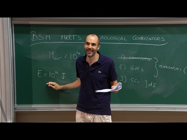
Raffaele D’Agnolo - 1/3 Beyond-the-Standard-Model meets Cosmological Correlators

Well, so thank you very much for the invitation. It's a it's a real pleasure uh to be here. So you as you have seen uh in many of the previous lectures, the sitter is baffling and amazing. So it can give you a lot of energy for free and that's exactly what particle physicist want. So in these lectures we're asking essentially what happens when they sit there and beyond the standard model or particle physics if you want to give it another name make a baby. Okay we're going to we're going to take a look at this baby and uh see if it breeds right and if it can tell us something about nature that we cannot learn in any other way. And uh well as an introduction let let me give you uh let's say some numbers as motivation. Okay. So let me be maximally ambitious and uh say that I want to probe the gut scale. Okay. So I'm a particle physicist. My goal in life is to understand what's the next layer uh in the description of nature. And uh as all of us in BSM, I like to play I risk I gain games. So I invent a model. The probability that it actually describes nature is very close to zero. But if it does, I get two Nobel prizes. So that's that's how BSM works roughly. And so but but you can see that that we are on a very small probability tale of a gosh for each one of the models. And uh well essentially at the moment uh we have uh no energy scale attached to a new description of nature that is guaranteed to be there. Okay. So we have some ins that there might be something at the TV scale. We have some ins that there can be something here. And then the only place where we're pretty sure that we're going to find something new is uh at the scale of quantum gravity at plank. But uh I would say that this scale is close enough and that that um we can start from here. So I would still call this a maximally ambitious scale also because if string theory or whatever UV completes gravity is weakly coupled then you're going to start seeing interesting gravitational physics already here. Um so okay so so let let's say I'm an experimentalist and I want to measure stuff at this scale. So what can I do? Well, I I I can build a collider. I can measure gravitational waves. Mainly I have in mind primordial gravitational waves that are produced early on in the history of the universe. So already the second route requires some luck. So it requires the fact that the universe existed at these temperatures and that something violent enough happened that we see it imprinting gravitational waves today. Okay, but let's let's assume we are lucky. And then the last thing I can do is is precisely uh measure this cosmological correlators. Okay, that I'm going to do some violence to myself and and and abbreviate as CC. But for me CC is the cosmological constant. I might confuse these two abbreviations in what follows. And uh well for the sake of the introduction the main difference between these three options is that these first two are in Minkoski if you want plus epsilon in the case of gravitational waves and this this other option instead comes from the sether and uh we're going to see immediately a big difference in how hard it is experimentally to probe the scaling minks versus the sitter in practice. this because uh well in this third case we're assuming that the sitter is already providing us with the necessary energy. Okay. So but but let's let's start from number one and keep going and see what's possible and what is not possible. So in the first case I want to build a collider uh at the gut scale. Okay. So I'm typically going to accelerate some particles in a circle and make them collide. So what rules my life is uh are Maxwell's equation or in this case the Lawrence fors. Okay. So if I want to put some particles on a circle that go fast enough well I need a big enough magnetic field. So you might think that the hardest thing to do if you want to build a collider at the gut scale is accelerate the particles at this energy. But actually the hardest thing to do is to keep them in an orbit and not lose them because well you can use this formula or its relativistic equivalent to get some numbers. So let's say I want a particle with momentum GV and I want it to be on an orbit of radius a meter and I can use a magnetic field of a Tesla. So this is the relation I get. And if now we put here say what I really want to probe and we put here say the best we can do now order 10 Tesla in a magnet. Well, we can we can actually do better. But here we're talking about building tens of thousands or hundreds of thousands of these magnets because well you what you're going to get immediately out of this formula is that you need a collider that is 10 par six long. Okay. So probably you're not going to do it. You can reverse this estimate. Okay. You can say okay the best I can do is a collider that is as big as the radius of the earth. So, so let's say something of roughly this size, okay, of 6,000 kilometers. Um, then what am I going to get out of it is that I need, let me see, I need 10 to the 10 Tesla. Okay, I think this second option is even worse. Okay, I I I think think I'm more confident that humanity can build a parcel clone collider than a 10 to the 10 Tesla magnet. probably it also goes I mean like there's no material that that will exist in this magnetic field. Okay. So so I guess that we don't want to go down this route. So then then at some point in my career uh I thought well I mean for sure it's easier to measure gravitational waves at 100 meghertz. I'm going to tell you in a second why 100 mehz or one ghz is the is the relevant number rather than building a gutscale collider. Okay, so in this case you just need to be very precise. Well, it turns out I was very wrong. Okay, one day I did the estimates and and in doing the estimates I kind of proven a theorem that's impossible to see gradational waves beyond a certain frequency. And I'm going to give you now let's say the twominut condensed version of this of this theorem. Um so okay what do you need uh if you want to probe mag gravitational wave? Well first of all you need to know what frequency you want to measure. Okay so and uh if you you can bound the wavelength of any process that occurred at some time in the history of the universe by the size of the horizon. Okay. So let's say you're interested in something that happened at some temperature tar. So in our case 10^ the 16 GV at that time observers could only see an horizon of order abble at that temperature. And so no process could exist with a wavelength bigger than than could be produced I mean could be generated with a wavelength bigger than the horizon. And so you can redshift this very simple uh estimate based on causality until today. And this is going to tell you what frequency you're going to measure in the lab if you want to see a graational weight produced at this temperature. So you're just uh going to redshift in the standard way with your scale factor and you're going to get that uh a gigz roughly the temperature that we want. If at the time you had something standard model like So these are the number of degrees of freedom that were acting were active at this temperature tar. So 100 is roughly the number for the standard model. But you see that the dependence is very mild. It goes like one over six. Okay. So let's say I want to prop this scale. Then I need to see gradial waves at a gigger. Can I do it? As I said the short answer is no. But let me tell you why. Uh okay so let let me just do the standard thing of breaking down the metric into some minkoski piece and a small perturbation. Okay. So, so this h is dimensionless and much smaller than one. Then I can expand my lranjon and I'm going to get the usual uh coupling between these gravitational waves and the stress energy tensor plus higher order terms in h plus derivative couplings in h. But what we care about in the end is how these gradation waves couple to our detector. So this is what's going to contain the coupling. And so very roughly we can estimate that this is going to give an effect that's proportional to h. So the dimensionless amplitude of the wave times whatever energy we're able to put in the detector. And you're going to see that you're going to need an energy that's not too far from this step to the well it's a smaller than 10 tesla but it's still way beyond what we can do uh as mankind. Uh so okay so at this point how do we do this estimate? So we just said that the the wave is coupling to the energy in our detector. So it's going to generate some signal power. This signal power is going to be well the energy the signal energy. So this is just whatever the graial wave is uh depositing into our detector times something with the dimension of time. And it's easy to show using pointings theorem. or really classical physics 102 that the biggest power that a signal oscillating at some frequency of a gas can have is this the energy times the frequency of the signal and then we're going to stick in there some uh some function that tells us how the detector responds okay and okay you might you might think that this this is the important part okay because this is what you get from dimensional analysis and usually as a theorist that's all you But actually we're pretty good at building detectors. So this this thing for the best detectors we have is like 10 to the 10 and we can even get to 10 to the 12 one day. So yes >> sorry without argue about this like this energy scale is still higher than inflation right but withination energy scale is 10 or 14 or something. >> Yeah. Well, yes, I'm being yes, maybe maybe I'm being overly optimistic in uh in getting all the way up here, but uh let's say that if you're completely agnostic about what happens to to quantum gravity at this scale or whatever happens before inflation. [snorts] Well, yes. So, so if you if you really uh so yes, so I would I would have taken a losser bound on inflation let's say than 10 to the 14 more like closer to 10 to the 16 and that's that's why I told you this number but okay I mean it doesn't really matter okay if we if you want we can scale it down by a factor of 100 and repeat all the estimates I mean what I'm trying to do here is just give you an idea that uh as you will see this is what can go highest in energy Okay. But uh yeah, so sure maybe my my my numbers on what's the latest bound on inflation were were not updated. Yes. Um all right. So okay. So now we have the signal power in the detector and we want to know if we can uh if we can uh see it. Well to know that we need some noise power in the detector. which is well it's at least one photon over the whole lifetime of the experiment. So this is how long you take data for and this is one photon. Okay. So you need at least this because even if you have zero noise okay if you are somehow able to set to zero even the quantum mechanical noise you still need to see one quantum to claim a detection. Okay. In reality, since uh this is our energy, so we're doing a linear experiment, you're going to have some of the energy that you put in the detector at the same frequency of the signal. So your background is going to be pluson with the number of photons that you put in your detector creating a source of noise for you. Okay, so this is a more realistic estimate. of your actual noise. I'm happy to go in more detail if it's not very clear, but uh if not, you can just I mean, if you don't want to ask anything, you can just trust me. If you're not notice that if you're able to put these photons exactly in the quantum state you want and keep them there this whole time, you can reduce this to zero. Okay, but this is uh as we will see at the end a completely impossible task at the moment. Okay, so this is let's say your smallest possible classical noise and by classical I mean that you set to zero all your other sources of noise except for quantum fluctuations but you did not set to zero the quantum fluctuations of the energy in your detector. Okay. So now we can just very roughly compare these two. So say that P signal over P noise has to be bigger than one. And then we're going to get some minimal H that we can probe. Okay, which is going to be of order if you do this ratio just 1 / square root of energy in the detector times time you run times one over the transfer function. Okay, note that already to do this estimate I've been rather crazy in some sense and you can see it if you restore units to H slash. Okay, so so if you restore units to H slash you get it here. So you see that essentially I'm comparing a pure quantum noise forgetting about everything else temperature vibrations everything that happens all the time in in the life of an experimentalist and I'm just using quantum fluctuations but even even so so even being this optimistic okay let's go back and say I want to probe this scale and I want to probe it better than existing cosmological bounds okay so to to see what it takes I need to translate this minimal strain that I can detect into an energy density. So let's say that the typical way in which these primordial backgrounds of gravitational waves are characterized is via this quantity omega. Oh, sorry. Which is just essentially the energy density in the gravitational wave normalized to the total energy density in the universe. Okay. So you can you can trade this parameter critical energy density for what Apple is today in this way. Okay. So for for now I mean we're just introducing a definition which makes it easy to compare actual experiments to cosmological experiments because cosmological experiments bound this quantity to be roughly smaller than 10 the minus 6. Okay. So now we want to translate that h down there into an energy density. And again okay I'm not going to show to you how it's done but roughly that's the result you get. So if you have a signal at omega s it goes like omega s cub times our h squ over well this is just the normalization coming from the definition times this delta omega which is let's say the the smallest between the frequency range over which the signal is spread and the sensitivity window of the detector. Okay, if we are maximally optimistic, we can take this frequency to be just one over the integration time. Okay, again I'm telling you this without proof because well this is not really the main focus of the lectures and I think I'm already spending too much time on it. So in the end roughly you're going to get uh this uh estimate for the energy density where this n is an order one number that depends on the geometry of the detector where the gravitational wave is coming from I mean all details that we're going to ignore. Okay. So now we can plug that h min into er and compare to the number 10 to the minus 6. Let's say we put here gigahertz. We put here um 1 / square root of energy time t in times one over this transfer function. For this transfer function we use 10 to the 10 which is the best we can do. Now [clears throat] this 10 to the 10 comes roughly from uh LIGO. So it's it's roughly the size of LIGO over the wavelength of the laser. This is an enhancement they get because they're measuring a phase. Okay. I realize I'm telling you a lot of stuff, but I promise that when we get to the to this part, I'm going to go much more slowly. Okay, so this is just a very quick introduction to give you an idea why this is roughly our only shot to pro very high energies. Um, okay. So, we put this 10 to the 10 transfer function. We put in gigahertz. That's what we want. We know what's the value of able today. And finally, let's say we operate the experiment for one year. Okay. Um yeah, so we want to do better than the cosmological bound otherwise the experiment is is useless. What we get is that we need 10 to the 14 jewles. Okay, this number maybe is telling you nothing but uh well probably 10 to the 14 is scaring you a little bit and it should because uh this is 100 times the energy that you need in the magnets of heater which is now the biggest fusion uh let's say enterprise that we have in the world. So doing something like this is not quite as extreme as having 10 to the 10 Tesla for the collider, but it's certainly out of the question anytime soon. If you want, let's say to keep a spec of optimism, if I imagine that I'm the god of quantum physics and I can put these photons not in a laser but in exactly the quantum state I want for one year, then this number is reduced dramatically. Okay, so you need only 10 theus4 jewles which you think okay I mean this is nothing. I'm sure that our quantum experimentalist friends can do it no problem. Okay, the problem is that if you translate this to photons at the typical frequency of a laser today, this is 10 to the five photons. And today our friends in quantum methology, quantum optics, they can maybe play with a few photons. Okay, I'm not sure of the exact number, but uh I I see I don't see this happening anytime soon. And even if they could okay so even if uh uh one experimentalist got got enlighted by the god author of experimental physics and tomorrow came up with a uh let's say a noon state with 10 to the five photons that he can control it would still be useless because at the moment let's say interferometers which are those that actually almost saturate these estimates they have optical losses at the level of 10 to the minus2 true which means that your perfect quantum state gets destroyed almost immediately and the performance of the interferometer is the same that I've estimated with this 10 to the 14 jewles. So if you want really to get here you also need to get your optical losses below one over the number of photons which again we have no idea how to do. Okay. So this is this was a very long way to say that uh you should probably forget also about this. Okay. Although you see they are kind of in order of how hard it is, but they are also in order of how let's say general they are. Okay. So the collider is really the best thing you can do because if you can turn it on, you more or less see anything that leaves at the energy scale where the collider is operating. The gravitational waves are not that great because okay, you need to be lucky. So they need to have been produced and they need to be have been produced with a huge amplitude. Okay, this 10 to the minus 6 can seem small but it's actually very big for a primordial signal. And now also we get to the last one. So the last one comes almost for free if inflation took place at this scale. Well, your colleague reminded me that the bound is actually stronger, but let's pretend that it's possible for a moment. Okay. So if inflation really took place at these scales then you can probe the scales at the cosmological collider but we're going to see I mean most of this this lecture is actually is going to see is we're going to try to see what we can probe and what we cannot probe. So how much we can learn on inflation at the cosmological collider and how much mo we can learn about particle physics. So let's even imagine that we are lucky and that inflation took place at these energy scales or maybe a factor of 100 below. Can we see anything? Well, unfortunately the answer will be again no. But we can see something. Okay, which is still exponentially better than the other two options. So I think it's it's a possibility that we should take seriously if we ever hope to probe extremely high energy scales. Um all right. So let's uh now forget uh yes >> just very quickly for this gravitational wave detection you're assuming you have some sort of electromagnetic system or something but imagine if you imagine that people actually made like bars work just have a very heavy mass change. >> Yes. So, so, so, okay, sadly in this in this detect, so, okay, yeah, it's funny because it's a very nice question because it allows me to to uh to say two things. So, one is that here I I'm already assuming that the mass of my detector is infinity. And the reason why it doesn't matter is because of the equivalence principle, right? So if [laughter] if you have say this is your your detector displacement from the equilibrium position is going to go roughly like gravitational mass times length of the detector times h double dot and so you see you send the mass to infinity and your signal stays the same. So, so essentially if you do that so if you send your signal to to your mass to infinity you are killing all the noise from external sources which is what I did there and then you are purely limited by the electromagnetic energy in the readout uh which in the case of LIGO is the laser in the case of the Weber bar they attach this uh resonance circuit to the bar that oscillates but then the estimate goes exactly in the same way except that here you have an h squ so it's it's worse. Uh well well it's not worse because here you have an H square but here you have only one photon because there is no interference. So in the end you get the exact same. However um what what you said is true in the sense that if you the best a Weber bar can do is better than the best that LIGO can do. Um so LIGO roughly saturates this estimate. The Weber bar is uh a factor I think 10 to the six uh worse than this estimate. If you wanted to saturate this estimate with a Weber bar, you would need a Weber bar uh roughly the same size of a medium asteroid. So maybe I mean maybe we can do it in space. I don't know. Uh but but note that again even if you do it, you just saturate my estimate. So you're not going to get to a gigahertz. Plus uh there is a limit to how big you can make the frequency of a mechanical resonance because the typical speed of sound in a material is like 10 the minus 6 to 10 to the minus 3. So Weber bars are typically going to work well at a kilohz but I know no material I mean so essentially you need a material that is as rigid as electromagnetic waves that I mean it doesn't exist. Um, yeah, if you want to do gigahertz. Uh, all right. So, um, so let's get to to the reason why we're here. Um, and so you'll see especially this first uh hour and a half. I'm going to repeat a lot of the things you've seen uh uh I think in the introductory lectures but I mean I find it's better to have a self-contained set of lectures and also I'm going to go very quickly on a few things so it's good that you've seen them already okay so okay the bas the basics of what I'm proposing to do is okay if you look at the sky the sky is almost homogeneous and isotropic but not exactly. Okay, there are some cold spots, some warm spots. And so what you can do is just look at the sky with your big sensitive eye and count the photons that eat your eye. If you do that, you're going to get some photon flux per unit area, per unit time, per unit frequency. And it turns out that you're going to see exactly a black body spectrum with some temperature. So you can measure. So doing this do this experiment just counting the photons that arrive to you as a function of frequency you're going to measure some average temperature of the sky. And then well you can repeat this exercise but now at fixed let's say line of sight. Okay, you ch you choose some point in the sky and then you can just compute the difference between whatever you see in a point and your average temperature. [clears throat] You do this, you do this for many different points in the sky and you then average over all points that have the same direction. Okay, so this is going to give you a sort of correlation function that looks like this. So you can choose however many points you want. In practice, we're very sensitive just to the twopoint function and to some extent to the three-point function. >> [clears throat] >> And this is going to be a measure of the energy density in the universe in those points. Okay. So I'm not so as I said at the beginning I'm I'm a particle physicist so I'm not really an expert on how this experiment work but that's roughly what the CMBB does. Okay. And you can repeat this also on different scales. Okay? So you can instead of uh counting bright spots and cold spots, you can count galaxies and do the exact same exercise. Okay? See how much energy. So there there's yeah, you're not going to map it to a black body spectrum as in this case, but you can still compute how much energy density there is in each point and build these correlation functions. And similarly, so so this would be large scale structure. And similarly, you can do it at yet different scales in the 21 cm line of hydrogen. So as you can see, I'm going very quickly because I'm sure you've heard this already in the past few days. And so these are going to be our three uh let's say year also. So the three experiments that can probe this uh these correlation functions in the sitter. And in practice what we're going to do is that we're going to start with the simplest possible scenario. Okay. So we're gonna imagine that at some large scale sorry at some early times high temperature the universe was dominated by a single scalar field. Okay. So, so we're going to assume that early on maybe at the large scale I drew I written down before at a slightly lower scale the energy density of the universe was dominated by the potential of the scalar. We're going to do this not because we woke up this morning so inclined but because this is the simplest model that describes very well all these sorts of observations. So if you assume that the universe was dominated let's say by the classical part of of this field and the classical part of this field was approximately independent of the space-time point then you're going to generate a universe that is approximately homogeneous and isotropic. So rotationally and translationally invariant but the quantum fluctuations of this field are precisely going to give you the bright and cold spots that we see in the CMBB and uh they're going to give you these bright and cold spots that respect the approximate symmetries that we see. Okay, so these fluctuations are going to be scaling variant adiabatic and gosh and we're going to see this in more detail in a second. So if this is the case, so if this is what actually happened at some point, then these uh fluctuations in temperature that we see today that are fluctuations in energy density can be mapped to the fluctuations of the scalar. So if uh if anything left an imprint on the fluctuations of the scalar, we can measure them today in this way. And uh well the interesting part is that uh we said that we're we're assuming that the potential of the scalar is dominating uh um the energy density of the universe at this early time. So if this is the case then we're going to be able to see anything roughly at this scale. So if you have a mass a passive particle with mass close to this double scale and it couples to whatever dominated the energy density is going to leave a trace in this uh in these correlators. It's actually a little bit better than this. Okay, because uh well there is also another scale in the problem which is phi dot and we're going to see in a second that this ph dot is bigger than abble order let's say it's order 60 and you can even probe particles of roughly this mass. Okay, so these are going to be our two main scales in the problem. Um so essentially all that we're going to do uh next is to make the statements more precise. Okay. And I'm going to take so now it sounds like I'm going to redo what you've seen in the previous lectures but I'm going to actually take a completely orthogonal approach. I think many of the previous lectures focused on the mathematical structure of these objects. I'm going to do the complete opposite. Okay, I'm going to forget about the mathematical beauty and detailed momentum dependence of these correlation functions. All I'm going to do is to set up a machinery that allows us to estimate very quickly the size of these objects so that we can estimate them in many examples and see if we can learn anything on the structure of this potential or if there are other particles coupled to fi or even more. Okay. Um, so the whole name of the game will be how can I estimate these objects in 3 seconds forgetting about all the details. Okay. Uh, but to do that we're going to start uh from from the very beginning. Okay. So I'm going to start by uh well making this lower picture a bit more detailed defining a few parameters that I'm sure all of you know but but it's always good to uh go through notation once more whenever one starts a new set of lectures. It's okay. So as we said this is the picture. Okay. Where The scalar is dominated by its classical motion. So you you write the lan equations of motion, you solve them and you get some some solution but it has some small quantum fluctuations and at least for some time the potential energy dominates the energy budget of the universe. So you see the apple parameter is dominated by the potential energy of this pi. to be consistent with these observations from the CMBB that I sketched, you need this to happen for long enough. Okay, so in practice, we're not going to be very precise on what we mean by long enough, but we're going to define as usual some old parameters and we're going to ask that they are much smaller than one. Okay, as again I'm going to go very quickly. I'm going to assume that you're more or less familiar with this picture. If you're not, please tell me and I can give you more details. So, we're going to ask that this parameter be small and also that this parameter be small and it's easy to show that you can translate these uh requirements on requirements of the potential of five. Okay, intuitively it's obvious. Okay, because you want this fi to roll slowly. So, you need the potential to be flat. flat in units of m plank. Okay, so this is not a very strong requirement for particle physices but still you can show that this epsilon is approximately in this simplified in this simple picture this quantity. So it's the first derivative of the potential and this EA is the second derivative appropriately normalized. So we want we want the potential to be flat and let's say also the acceleration at a to be small. If all these is satisfied as I was saying this uh this quantum fluctuation wells are going to take care of uh of describing the temperature fluctuations in the CMD. Okay. So this is let's say the the basic setup. So we're going to imagine that a period like this took place at some time in the history of the universe. Uh and now we want to compute the correlation functions for these fluctuations delta fi. To do it well it's convenient to first of all do it in global deer coordinates introducing conformal time. So instead of using say the normal FRW metric that we typically use in cosmology, I'm going to introduce conformal time. So our scaling of time by the scale factor and we're going to work in these coordinates. Then we're going to go to FIA space because well as we said multiple times the universe is approximately homogeneous and isotropic on large scales and so well going to Face and forces in a simple way translational and rotational invariance. And then finally well we're going to split all quantities like this. Okay. So the scalar fi has a background and fluctuations but but this implies that also the energy density has a background plus fluctuation that also the stress energy tensor that also the metric because the metric is sourced by the stress energy tensor of the scalar. And I'm often going to forget about the bars. So if you see a quantity that doesn't have a delta it's a background quantity. Okay. Um the last thing that we need to do is uh make the calculation gauge invariant. Okay. So we've been very loose in uh talking about the fluctuations of the scalar, the metric, the energy density. Well, it's this is because I mean if you choose a gauge, you can move the fluctuations from one to the other. So the the the sensible thing to do is to work with a gauge invariant quantity. And I'm going to work with this zeta which is defined in the following way where uh sigh is a fluctuation of the matrix. So if we write the special part of the matrix, this side is just one of its scalar fluctuations. Okay, [clears throat] as you pro some of you probably have seen uh a million times, what's nice about this Zetta is that not only it's gauging varant, but it also uh stays fixed after it leaves the horizon. Okay. So if we go uh to fa space and consider the free compon component of of this quantity and write this equation of motion it's going to look schematically like this. So this delta a is zero whenever this is true. So whenever the fluctuations of the stress energy tensor are adiabatic, I'm not going to prove it to you, but uh if you actually start from this action and compute the stress energy tensor, you're going to find that for a single scalar field dominating the energy density, this is true. Okay, so we can forget about this part in the time of evolution of our zeta and this part becomes zero when the mode exits the horizon. So the k is the inverse of the wavelength of the mode. So whenever the wavelength is small and the mode is in so the horizon is roughly of size a h. So whenever the mode has a wavelength within the horizon, this thing is evolving. But when the wavelength of the mode becomes bigger than the horizon, it's frozen. Okay. So we're going to have a series of uh of quantities that we can measure that have memory of what happened very early on in the history of the universe. So they exited the horizon at some point during inflation and then they are re-entering the horizon today. And so by measuring correlation functions of this data, we're measuring a snapshot of the universe during inflation. Okay. So again, this was all very quick, but because I'm assuming you've seen it a few times already. Um and as usual well in quantum field theory we more or less how to know to do only three fields. So so the first step is to compute the twooint function. Okay. So we want to compute this quantity that we're going to use to normalize everything else. Then the real let's say main character of the lectures will be the threepoint function but it's useful to start with the let's say free part of the field which is also the one that we can measure best at current experiments. Well, if you want to if we want to compute the the twooint function, we can start by rewriting our action in terms of zeta and expanding it to second order. Okay, so we take the same action, we plug in the definition of zeta and we expand it to second order. This is actually quite a bit of work if you want to do it, but it's a nice exercise. So this is a scale factor cube. This is fi dot evaluated on the background. Apple evaluated on the background. And then here we have our fluctuations. So the reason why expanded the action is purely dictated by observation. Okay. So today in the CMBB we see something that looks roughly like a free field okay with very small perturbations on top. So this zeta is measured in the CMBB of being of order 10 to the minus 4 roughly and so whatever higher order temp that could be there might be there but uh it's right at the boundary of our abilities to see it. Actually the the whole thing we're going to do in this lecture is to check check whether we can see any of these of these higher order terms. Uh but okay so so this experimental fact is actually helping us a lot because uh now we have a quadratic action and we want to compute a twopoint function. So if you allow me to go to go to the ukidian all that we're doing is solving a gosh integral. Okay. So we're computing this zeta squared which is just a gosh pat integral where this o is some differential operator that you can read out from this action. Okay. And it turns out that the gosh pat integral is practically the only pat integral we know how to do. And uh well you wouldn't be surprised to know that the result is exactly the same as the normal gosh integral. So if you're able to compute the inverse of this operator then you also know the twooint function. Of course going from here to here contains infinitely many subals subies I mean. So what contour do you take to invert the operator? So you can get a million different answers if you're not careful. Okay. Again, in the spirit of this being a quick introduction, I'm going to gloss over all the scientists and just show you the fastest possible way to get the right result by just using dimensional analysis. Okay, so again, we forget about mathematical beauty. I'm I'm sure that many of you are in pain right now, but don't worry because you will be way more in pain in a second when I'm going to do all integrals using dimensional analysis. But it it gets there. It gets it gets the job done. Okay. So what is this guy O? Well, we have to get it from the action. And in particular, well, we need to do the integral. And here is how I'm going to do the integral. So for me, the integral over space is 1 / k cube and the integral over time is one over. Okay, so these are the only time scales I have and the only length scale I have. If I'm interested in the twooint function of ZK K prime, why K and not K prime? You ask me, I answer translational invariance. K and K prime need to be the same or the function is zero. Then what else am I going to do? Well, I have the rest the rest of the operator ER and I'm just going to focus on the space derivative. The other piece gives the same. So the rest of the operator here is a cub * 5 dot 2 over a squar time um 1 / a^ 2 and a time d sorry a space derivative squared again so I'm going to estimate space derivatives by k. So this is gives giving me a k squ and I'm interested in evaluating this expression at horizon crossing. So when k is approximately equal to the size of the horizon. Okay. The reason being this one that what what we're measuring is z the moment it exits the horizon. Okay. And so this gives me for this quantity um well so let let me actually add everything okay d3x dt. So this is really my O okay quote and quote okay and this gives me 5 dot 2 over h 2 1 / h 2 so we are almost there of course never do this at home okay these estimates are dangerous things to do I'm just uh giving you a feeling for why you get the result you always get. Okay, but this is what the FIA transform of my position space um twooint function. Okay, so of my zx zy that I was computing from my uklidian party integral. Okay. And so now, okay, we said that this is O to the minus one. So I'm just going to stick my estimate for O to the minus one. But I need to do the integral. Okay, one is giving me a delta function because of translational invariance. The other one, well, I brutally estimate it in the same way as before. And finally I get the right the the final result. Okay. Oh, sorry. That's it. Notice that I could argue again without doing the calculation that I expect the time derivative that I did not use to give me the same result as the space derivative. If I if I do that then O should be twice that roughly and I'm going to get the following result. Okay, from my estimate the 2 pi cube coming from the um integral over the exponential this turns out to be exactly the right result even at the level of the factor of two. I have to say I was quite amazed after doing this super rough estimate to get the right result but you shouldn't be amazed to get the right parametric dependencies. Okay. Uh so okay so this was just a fun exercise to make everyone in the audience that's more mathematically minded feel terrible but also to give you a flavor of what's coming next. Okay. So this is what we're going to do next. So, we're going to trying to find the dirtiest and quickest possible way to estimate higher point functions to see if we can say anything about inflation or particle physics. Um, one thing that we can check about this estimate well is that it's scaling variant. So, this 1 / k cube as you probably know is kind of the hallmark of scaling variance in four dimensions. The reason is trivial. It's just that okay. So do a do a scale transformation. You can check immediately that what generates this is uh in our coordinates an operator that looks like this. Okay. If you fur transform it, you're going to get this. And so this three this one over k cube is exactly what you need to get something scaling variant. So if you act with the our fier transformed operator on our twooint function you get scaling variance. Okay. Well let's say the primed one without the delta function from translational invariance. All right. So uh we're almost done let's say setting the stage. So this was just to set the notation and uh and make sure that we were all on the same page uh to finish setting the notation. Well, so what's next? So what's coming next is that we want to compute these three point functions and we're going to normalize them in this way. where pz pz is uh essentially proportional to the twooint function that we just computed. So you remove the k dependence and the delta function and add a 2 pi squ. So the reason why we chosen this normalization is uh that we can very roughly say that uh what we measure in the experiment so the amplitude of nonausianities that I'm going to call FNL and I'm going to in a second give you a few disclaimers on what this FNL means. It's roughly the let's say the magnitude of this function S. Okay. So in what follows we're going to forget everything about S and the fact that there are three momentum. Okay. So we're always going to normalize everything to the largest momentum if the in the problem. Let me call it K and then have let's say functions of dimensionless uh ratios. Okay. [snorts] So, in practice, what we're going to do is uh measure. So, we're going to let me delete a few things. So what we're going to do is start with some action for our inflate inflaton fi. We're going to introduce essentially standard pat integral techniques to compute the correlation functions of phi mainly this threepoint function. Okay. And then we're going to convert this well into a threepoint function for zed from which we're going to extract this FNL and compare to experiment. Okay. So, this part is the one that requires uh the largest amount of work, and we're probably going to do it uh the next in the next round, but we're going to start. Okay, but we're going to do it in the next round. These two parts instead, since I'm doing them super roughly, are very easy. And let me tell you how they're done. So first of all okay you can recall the definition of zed if you use the action for the single inflaton that we written down before you can show that uh in this lower regimes regime that we described so epsilon and are much smaller than one. This is approximately true. Okay. Then we're going to work in a gauge where size is zero. And this is simply going to give us that zed is roughly minus h or phi dot delta fi. Okay. So from here we see that our let's say rough estimate for fn so the magnitude of that function s can [snorts] be written in terms of uh the correlation function of delta ph in the following way. So and this prime means that I factored out the delta function from momentum conservation. Okay, from translational invariance. Let me maybe write the next formula in a more prominent place because we're going to use it all the time. Okay. So now well we can use uh we can use uh okay this definition to simplify this relation and finally we're going to get that the quantity that we're interested in for experiment is roughly k to the 6 times 5 of k1 k2 k3 3 over P of Z to the 12 * A cube. Okay, so we're going to use this all the time to estimate our experimentally relevant parameter and we're going to also use that this speed z is been measured by flank to be roughly 10 3 * 10 the minus 9 which from the definition this implies what I was telling you before that five dot to the 1/2 is roughly 60 times probably before I think I I wrote PH dot equals 60 times double. That's obviously wrong because phi dot is an energy squared. Okay. Um okay. So I think we have roughly all the ingredients uh to start uh our journey. Uh the only other thing I want to tell you is roughly how well we can do experimentally on this FNL. Okay. Okay. >> Yes. >> If the is 10 minus 5, wouldn't the estimate be 10 the spectum is 10 - 45 times the power? >> Sorry, say that again. The >> zeta is 10 - 4 just be 10 - 4 times the power spectrum. >> Uh yeah, yeah. So, so indeed indeed you see I normalized it to the power. Yes. So it should be the roughly the power spectrum squared. So that that's why I normalize it like that. So so roughly roughly so I roughly expect Zeta Q. So I roughly expect this guy to go like this roughly. Okay. modulo modulo the the dimensions of K. Okay. This is >> and yes >> you lost me a little bit on this last action as >> I no sorry this is not the action. Yeah, actually this is a terrible Well, let me call this A. Okay. Yeah, sorry. I I should not call it S, but it's called S a bit everywhere in the literature. So, so this S. So, this S that now I'm calling A is just this function of momenta. Okay, it's just whatever is left of the threepoint function after I factor out the dimension full piece and this PZ squared the normalization. >> Okay, and then to get to the next line the next >> this line. >> You're solving for >> Yes, I'm solving for a >> solving for a and then I'm using the relation between zed and delta. Yeah, that's it. Um, yes. Okay. So, so to to to conclude this very long introduction, um, let me say something about the numbers. So, so a disclaimer is that the numbers I'm going to tell you should be taken with a grain of salt. Okay? So, the CNB can do roughly FNL of order five on something called local. So usually FNL is defined for for the so-called local nongianity which is a a particular choice of uh of the functional form of this a okay and this is roughly the best that the CMB can do right now. Okay, some people have actually tried to recast plank data uh on uh some signal that could come from new particles produced during inflation and they're getting something more like 40. Okay, 40 at one sigma. So order 80 at two sigma large scale structure. Well, we hope it can do order one based on cosmic variance, but then okay, if you're optimistic and again you you look at the local one and combine CMBB and large scale structure, you can maybe get to 0.1. But so you you see these number mean very little because they depend a lot on the special function that you choose and they don't really want to specify a function. Okay. So I'm giving them to you. So you're not completely in the ocean of having no reference. But you should keep in mind that as this function changes what an experiment can do can get worse by a factor of 10 easily. Okay. And for 21 cm again I've seen all sorts of numbers floating around ranging from 10 to the minus2 to 10 the minus4. This is partially also because uh well we are not sure exactly how well the experiments can do in the future but I'm far from being an expert on any of these. So please refer to whatever numbers the previous lecturers gave to you. Okay. This is only to roughly anchor what we're going to get uh next in some in some examples to roughly what experiments might be able to do. Okay. Okay. So, uh what are we going to do uh next? So we're going to do a very quick introduction introduction to swinger calish essentially okay you've seen this already I think to some extent all we're going to do is uh to give you an idea on how to be able to estimate these quantities using fman diagrams essentially okay so that that's the goal of this introduction to swinginger Kelish which you can call Zwinger Kish for people that already know how it's done. Okay, because it's going to be very fast. Then uh we're going to ask what can can we learn about inflation by measuring these three point functions. Okay, more precisely, we're going to start by this very simple model that uh I sketched on the board for you with one field and then we're going to ask what can we learn about particle physics. Okay. with this being maybe my favorite part because okay, I'm going to I'm going to try to kind of get outside the language of cosmological correlators to make analogies with things that were already well known. Okay, because a lot of the things that we can learn about particle physics from cosmological correlators uh were phrased 30 years ago in a different way and and it actually helps a lot to build intuition to move from one language to the other. So a lot of things that you can see in cosmological correlators. You can also see it from the perspective of the sitter being a thermal bat with some number of particles floating around or from the point of view of uh producing particles during inflation from what people used to call preheating. So having some sort of parametric resonance in the equation of motion. So we're going to in this let's say last part of the lectures we're going to go back and forth a lot between the language of these correlators and some more old-fashioned language. I think this helps build some intuition. Uh how much time do I >> 20 minutes >> 20 minutes. Okay then. Then okay then I think we have we have enough time to start at least uh the first part. Well, as I said, I think you've seen this already. So, I'm going to try not to bore you. So, what we want to do, so we just said that at some point this perturbation exit inflation and then we measure them today. So, in practice, what we're measuring are correlation functions of field at a fixed time. So all the fields in this correlator are evaluated at the same at the same time. We're going to call this for varity Q of toao. Uh if possibly these fields can have some internal indices that distinguish between different flavors or different quantum numbers. But uh well it's not going to matter for us too much. And so the first thing that we're going to do as usual is to insert the identity written in terms of some uh some complete set of states at some time that we're going to call to final. Okay. So this is uh the last time um in our calculation. Okay. So let's say the moment where these objects exit inflation. So we're going to put our identity here. Uh what am I doing? Yes. The reason to do it is that uh well we know how to compute in out correlators and this is mapping our problem of computing a correlator at fixed time between two vacuum states defined also at the same time into computing some in out type of matrix elements. So these are at some time to f that we are going to choose to be larger than the time at which we're evaluating the fields in in such a way that we are we have mapped our calculation into an inout calculation and we see immediately that I mean this trick also shows you that this thing is observable at least at an intuitive level because it has the form of a cross-section you see. So it looks like a a matrix element an amplitude squared. [snorts] This is all very rough but again I'm assuming that some before me gave you the more uh mathematically uh rigorous picture and then I'm going to do one more thing. So now I'm going to foliate space time between some initial slice at time to zero all the way to my final slice at time to f into a bunch of slices and at each time slice I'm going to have a field five and I'm going to have a conjugate momentum to that field defined in the usual way to the Hamiltonian and in terms of these fields I can again write some sort of formally some identity as a sum of all the states of the field operator and I can also have another way to write the identities the identity in terms of the conjugate moment So this is more or less the standard way in which you go from some some amplitude to a party integral. And if I insert all these sums into my expression above and take the limit for uh the slicing to become very dense, I end up with a pati integral. So let's uh but let me do it separately for the two pieces. Okay. So I'm going to insert the identity in the two pieces separately and I'm going to evaluate them one by one. Let me delete this. Okay. So [clears throat] my amplitude here on the right hand side after this procedure becomes a part integral over phi n pi I'm going to call them plus because this matrix element has the structure of a time order correlator. So the out state is on the left, the in state is on the right and I'm going to need instead an anti-time order but integral to do to take care of the other matrix element which is um flipped. So this this integral comes from the sums and then I'm going to get a factor of e to the i integral between my initial and final time and integral over all of space of pi plus time 5 plus where this is the derivative with respect to conformal time. If I'm adding indices uh to these fields, I also have to sum over the indices. So you shouldn't be surprised to see this term appear after I introduce the states because it's just it's just coming from the the products between the states of the field operator and its conjugate momenta. Okay. So this should be familiar to you from quantum mechanics. So if you take position and momentum and compute these matrix elements, you're going to get things that look like this. And that's exactly what you're getting here. Okay, so this is the origin of this term. And then you're also going to get an amonian written in terms of these pi pluses and pi pluses. The Hamiltonian just comes from the fact that the state of the field operator at time toao is the time evolved uh state. Okay, so sorry. So that this guy is just the time evolved of whatever state you had at time to zero. Okay. So again, I'm doing things very roughly, but the goal here is to give you an intuition for where all the pieces are coming from. Uh and then well here I still have my product of fields so that I've called Q of TOAO. So here I still have my Q of toao. And finally uh I'm left with my let's say out state time 5 plus at the final time times 5 plus at the initial time times my in state. Okay, so I didn't do the full calculation for you, but if you just insert those complete sets of states inside, that's exactly what you're going to get. All right. So, this is a bit the most boring part of the whole story. Uh since I'm not doing it in the proper way, but uh if you bear with me, then we're going to develop a machinery with which we can have some fun. [snorts] uh and maybe I should have said it at the beginning but the goal of this whole procedure will be to show that this guy gives a part integral that's almost identical to the usual uh part integral that you use to compute cross-section. So you're going to have some lagran here at the exponent only it's doubled. So you're going to have the plus fields and the minus fields for this other matrix element. And then in practice once we get to this party integral with the lranjan at the exponent we can just use all the usual final machinery of diagrams to compute the correlation functions. Uh and so so this this this intermediate steps are what it takes to get there. Okay. So to get from the in in amplitude to a party integral that looks falike. Let's say you can do the exact same thing for the other matrix element and you're going to get another path integral. So these minuses are just names that were given to these other fields with the same exponent. Not surprisingly. Um well this time there is no Q but you still have uh this uh oh sorry what am I doing? Oh sorry yes you still have this uh product of amplitudes here. All right. So now we take our two part integrals, we multiply them and sum over alpha. Sorry. Well, what we're going to get is the sum over all of them. So, the integral, sorry, over all of them. We're going to have our Q of toao. So, all these fields, we're going to have the two exponents. Okay, I'm not going to rewrite them. It's just the sum of the two exponents. Uh, and then what survives summing over alpha is this. It's a sort of wave function of the vacuum. Okay, [snorts] or or rather a product of two wave functions of the vacuum. So since we're summing over alpha, you see you're going to end up having a fi plus dotted into a fi minus. So a fi minus at the final time dotted into a 5 plus uh also at the final time. And this gives us a delta function of uh 5 plus at the final time minus 5 minus at the final time. Okay. So this is just telling us that the plus and minus fields have to be the same. on the final time slice. Okay, so at this point we are almost there. So now we have to say something about the amonian or the lranjon that we started with. Okay. If it's quadratic in derivatives, then it's going to be quadratic in the pies and we can do the integral exactly. If it's not quadratic in derivatives, it's not quadratic in the pies and we don't know how to do the pi integral explicitly. But we can do it perturbatively. Okay. What I'm writing next is strictly valid just for uh uh amiltonians or lranchions that are that have at most quadratic terms in derivatives. But you can show perturbatively that the result is good at least up to order four in derivatives. However, you should keep in mind that exactly like in flat space, there are theories with many derivatives where this fails. Okay, you could just not use the pat integral in terms of the lranjon to get the fine man rules and get your correlators right. Okay, when you have many derivatives, you'd better do the usual ailonian calculation in the interaction picture. uh but for all the examples we're going to do in these lectures, this is not going to matter. So I'm just going to happily gloss over this complication and do my integral over the pies assuming that uh the Hamiltonian is quadratic in derivatives. Okay, if you do it, you're going to get the result that we were hoping for. So something that looks a lot like a party integral where this is the lranjon density. Okay, the two have the opposite sign because as we were saying we're computing let's say a timeordered amplitude and an anti-timeordered amplitude and then well we are left with the delta function that I'm not going to rewrite because it's just a prescription essentially the delta function is just enforcing some boundary conditions okay so I could even just not write it down but evaluate the party integral with the boundary condition that 5 plus at the final time is equal to 5 minus at the final time. Okay, so let me drop it for simplicity but I am left with a sort of unwanted piece which is 5 minus of 0 times 5 + 0 Okay, so if you're familiar with the usual pat integral story in flat space, you know what this is. Okay, so these are two sorts of wave functions of the vacuum that are going to tell you what's the right contour in free space to always the propagators. So these are the Iapsilon and well I'm going to show you in a moment if I have enough time or or uh >> yeah like five minutes >> okay well I'm going to start showing you and then we're going to probably finish uh um this afternoon I should say that okay this very rough uh derivation that I given you you can find it uh done more accurately here for example. Okay. Or you can just look at Weineberg quantum field theory one to get the same for in out correlators and the steps are almost identical except for the doubling of the fields. So if you want the really in-depth discussion go to weineberg. Um, all right. So, we want to evaluate this object. And again, I'm going to emphasize intuition over accuracy. Okay. The way you do it is that uh well, despise we can de compose them as usual uh in fier modes. Okay. All right. that then and when we quantize the theory these three modes become anation and creation operators. Okay, this omega is our vacuum. So it's only natural to ask that all the anilation operators set the vacuum to zero. Okay, okay, that that should not be an issue. But now we want to evaluate the product of the vacuum with a with a field I guess state. So it's useful to rewrite this annulation operators as sort of linear superpositions of of the field plus its conjugate momentum. Okay. So [snorts] you can easily invert uh this relation and whatever you get for the Hamiltonian for pi to write down the annulation operators. So I'm not going to I'm not going to do it for you but uh it's obvious that it's a linear combination of phi and pi. Okay. Um let's let me be just slightly more precise and say that uh okay you can write this as uh phi and pi in space for a transformed. Okay. But then uh well again here it would take some work to really prove this but it's a rather well-known fact that again should be familiar for from quantum mechanics that the conjugate momentum of an operator acts on the states of those of that operator as the derivative. Okay. So in practice we can turn this equation for the AKs that annulate the vacuum into a differential equation for this quantity in the following way. So you have say five plus of to zero a of k acting on omega is equal to zero. Now we plug here our solution for the annulation operator in terms of the field. Uh sorry this should be uh x in terms of the field and the conjugate momentum. And now, as we said, the conjugate momentum acting on the field states acts as a derivative. And so, schematically, you're going to have something that looks like phi. Now, so let me call this let's say fi tild. So that's it's clear that it's the value. Okay. So now this this phi here it's a quantum field and this pi is a quantum operator. But once they act on the state well phi becomes just a c number function. Okay. and uh pi just becomes uh functional derivative but again a c number let's say functional derivative uh here okay there are coefficients that I did not specify and there is okay this uh this sum over space-time points times the fia transform and all this operator is acting on our amplitude Okay, that as I said we can interpret as a wave function of the vacuum. So now we have all our operator that is acting on this wave function. So it turns out that this is an equation that we know how to solve. Okay. With aosians. So we're going to assume that the equation looks like this where sorry the solution looks like this where n is some normalization factor. And then we can plug this solution back into the differential equation and solve for E. And you're going to find that E. Is this This is if you have only one species of field. If you have internal indices, you can add them here and here you get a delta AB. Okay. Now we are almost uh almost done. Okay. We're going to take our initial time to minus infinity and use a relatively standard trick which is valid for sufficiently smooth boot functions. So we're going to write the function evaluated as minus infinity as the limit for epsilon that goes to zero of this integral. And if we do that [clears throat] we can promote we can add here an integral over time. Okay. So, we're going to have that uh that our e goes to itself integrated over time. Uh sorry, I think I forgot an epsilon. Yes, I forgot an epsilon. time epsilon [snorts] from minus infinity to let's say to to the end of inflation. So we're going to set so so we set the initial time to minus infinity and we're also going to set the final time at the end of inflation at to equal zero. And so now we can promote this e that was an integral just over over fa space to have also an integral over time. And this is useful because once we plug back here the solution that we have found. So this this gshian answers with e written down in this way. Then we're gonna find that [clears throat] all we did was shift the lranion of the timeordered fields by a small infinite decimal quantity. team. He All right. So you can do the exact same thing for the other term and we're going to and you're going to get that the lranjon for five minus is shifted in the same way with a minus here and minus 5. And finally, well, this I'm not going to show it to you, but uh again, you can go back to Weineberg and show that this is equivalent to an analytic continuation of time. For example, going to 1 + i epsilon toao for the five plus and minus for the five minus. Okay. So essentially as we were saying at the beginning and apologies if I'm not showing you this in detail but uh time is running out. This factor here is just shifting the lranja by an infinite decimal quantity which is essentially telling you which is the right way of computing timeordered and anti-time order correlators. Okay. In practice, from now on, we're going to forget all this and just uh start from uh this final result so that our incorrelator can be written as a part integral. I'm going to write here I epsilon as a subscript of the lranjan to remind myself that these uh two matrix elements are telling me which which is the right way of computing the time order and anti-time order correlators. But now we are armed with a part integral that's apart from the duplication of the fields identical to the usual one and we can just reuse all the fman diagram machinery to compute correlators and that's what we're going to do next. uh if we have time uh I will start by reviewing very quickly perturbation theory to show you why essentially using this part integral to do perturbation theory it just amounts to multiplying propagators and then we're going to get into it okay we're going to start computing these three point correlators using diagrammatics estimate their size and see what we can learn about inflation and particle physics okay so I'm glad we got through the more most painful part now so that this afternoon we can have more fun. [applause]