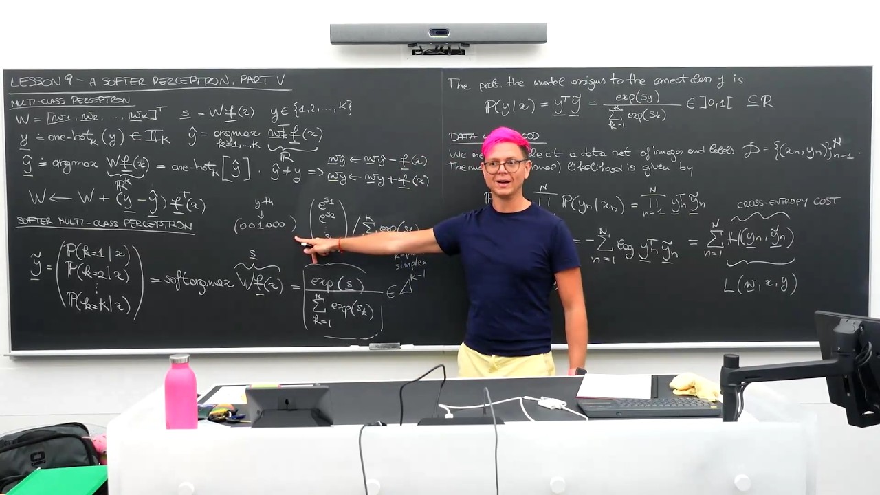
Lesson 09 – A softer perceptron, part V: multi-class likelihood and loss

Anyway, so let's see how to do exactly the same thing we have seen today in the quiz in the on the blackboard, but for the multi case version, okay? Which you can guess is going to be exactly the next quiz. So, the next quiz is exactly the same, right? So, if you didn't get it right this time, next time it should be perfect. All right. So, where are we? NYU now. That's um nine again. So, soft perceptron. This is part five. That doesn't finish. This is soft third. All right. So, very very very quickly, let's recap what we have seen in the case of multi class classification. So, we have multi class perceptron. We said we have a container for all my weights. How many weights I have? Eight, right? So, this is going to be my matrix where each row is going to be one of those weights. All of these are vectors. Then we were computing our projection and our inner products. So, we have my vector and I'll be equal to the multiplication of this big matrix time my feature for my specific this case image representing my, for example, digit from zero to nine. So, I have 10 possible classes, for example. Then we said that So, X is the digit, then we also have the Y. Y, what is Y? So, we introduce a new Y. Y was the class. Remember, in this case, Y belongs to, for example, 1 to capital K. And then I introduced something else, which was the Y with a bar underneath. And so I have my Y with a bar, which is defined as my one hot out of capital K elements of my scalars Y, right? So Y is an integer 1 to capital K. The one hot with capital K components is going to be one of the column of the identity matrix of size by the identity The matrix has all zeros but a one in a specific location. So the one hot of this integer here is simply the whatever case column of this identity matrix. Okay? I know you cannot really write this, but don't really care. So something I did forget to mention last time was the following. So last time I also mentioned how did we find a prediction for this multi-class perceptron? The multi-class perceptron, since you have multiple of these inner products, the winning class will be the class associated to the largest inner product, right? And so we said that Y hat was the argmax over lowercase one goes from one to capital K of all those inner products. Right? So you perform capital K inner products, and then my solution, my output, my model prediction that is associated to the inner product which has the largest value. And then I didn't tell you what was Y hat with a bar underneath. Can you guess, although I didn't tell you? What is the Y hat with a bar underneath? >> The one hot encoder of argmax of this. >> Right. So that would be the intuitive definitions, but I didn't say. So I that if I don't say something can I can leave room for confusion. So, let me actually make it explicit. My Y hat with a bar underneath is going to be and I call it here as a definition, the argmax of the this over here, okay? So, what am I saying here? This argmax doesn't have something underneath because it operates on a vector. So, meanwhile here, this thing here is a scalar. This is actually well, it's a scalar index indexed scalar. So, this is an indexed scalar. This is a a vector of capital K components. So, the argmax is going to just pick the largest of the K components in this case. That's why there is no index running index here. Meanwhile, in this case, the argmax of a scalar function, I had this index K and that's why I write here all try all possible K's, okay? Yeah. >> Should it be f of x? >> That is correct. Yes, I am getting confused. Thank you so much. Yeah. So, how do we define the argmax of a vector? As you just pointed out, this is going to be simply the one hot capital K of exactly this thing here, right? Of the one Y hat, right? Okay, but now we have this additional thing, right? So, we're going to have the argmax of a vector which I didn't really define. Okay, so given this, what is the update rule for my multi-class perception? So, we have we the two update rules. So, if Y hat is different from my target Y then I had to do two different things. It means that the inner product for the this guy is larger than the correct one. And there I have Therefore, I have to lower the inner product for this guy. I do that by taking the Y associated to the largest inner product and I try to make it smaller by subtracting feature vector. And then I take the Y for the correct class and I try to increase that inner product by adding. This is for the case where I deal with the individual item one at a time. I can just put them all together as we saw at the end of the last class. We can just take all these Ws, update them with the previous W value plus the difference between Y and Y hat vector multiplied by the feature vector. And we have seen that this thing here it's what type of product it is. It's the outer product. The left-hand side is a column vector. The right-hand side is a row vector. So, whenever you multiply those two things, you're going to get a box the same size as W. And so, whenever you're doing this addition, you will add the feature vector at the correct weight and you will subtract the feature vector in corresponding to the most offending class. We already seen this from the last episode. I'm just reviewing the content by an additional definition. Okay? All right. So, then we decided to go for the softer version that we have here. The softer multiclass perceptron. So, what is the only difference here? The only difference is going to be how I compute my prediction. So, I will start using vectors. So, we instead of using the Y hat, I'm going to have the Y tilde. What is the Y tilde? Y tilde tells me what is the belief of my model that that specific image belongs to any of the 10 different possible classes. And so, we have in this case my Y tilde is going to be a vector of probabilities that is looking for the first class for my specific image. Probability for looking at the second class for the given image up to the last probability that I'm looking at the last class for my image. And so, how do I compute this bunch of probabilities? I can compute this bunch of probabilities by using >> Softmax. >> the soft version of this guy here. So, everything makes just sense. I hope. If it doesn't, complain. Right? This is the hard argmax. Here, I just use the soft argmax. And so, here I will use this word, which is the soft arg max of what? Of the same thing, right? Here, this guy here. W F of X. So, we said this is going to be my S vector. We define it here. And so, if I have my S vector, what is the soft argmax of the S vector? It's going to be the exponential of the vector, which is going to be all the exponentiated components divided by the sum of all its components. This thing here on the top is the vector e to the S1 e to the S2 e to the S K. So the numerator is a vector then I divide by the sum of all these components. So now we're going to be moving forward and asking ourselves what is the probability for the class Y. Here I have all classes. This is class one, class two. K stands stands for class. I don't use C because C stands for cost. So we use K for class. So how do I find out the probability for the class Y? Y is the correct class. Can you tell? Can you tell me? Yeah. One hot encode Y and take the inner product with Y children. Yes, did I already show you that one last time? No. No, okay. How do you know? You just know it. Cool. That that's sweet. All right. So what what is going to be the probability the model assigns to the correct class Y is We write it here. Right. So I just extract. This is one hot. I multiply row times column. I just extract the Y's component of this thing over here. And so if I if I just do that, right? Here you have a vector. Which one comes out? If I have a vector I multiply that by a one-hot vector, which of these exponentials will jump out? >> The one with the one. >> Exactly, right? So, I write it here. It's going to be exponential of the SY. So, this is a scalar. Then I divide again by all those guys, right? Okay, cool. So, now we can get the second part of today's today's topic, today's class, which is exactly going through the same questions we have seen on the quiz, right? So, they they can write in there. So, we have a data set, right? We would like to eventually find our weights, right? Here we had the update rule for the multiclass perceptron. >> Yeah, what's up? >> Yeah, so we had a on Y field uh underscore, we had an initial exponent of Y as the top part. Yes? There. Exponent of S. But there we go exponent of SY. How was that transition? Like, how did it happen? >> What is this guy here? >> It's one-hot encoder. >> One-hot. You multiply one-hot times this vector. What do you get? >> One-hot times this vector. So, one-hot is a value of a one where the class is correct. >> Yeah. >> So, you just get to >> What happens if you multiply those two things together? >> So, you get one element, each of a power of S. >> What happens if you multiply this times this? >> Matrix multiplication. >> It's a row vector times a column vector. Yes, what happens if you multiply this single row times this? >> the one by one. >> I get a one by one which value is? >> S index Y. Thank you. Yes. >> And that's what's written over there. Amazing. Cool. >> index Y, right? >> That's index Y. Yes. Yes, it's an index Y. It's a bit bigger because you cannot do it over there. Yes. >> Over there you do Y transpose times Y tilde on the numerator. On that one. You did times Y tilde. >> Yeah, and Y tilde is that, right? Yeah. >> How do you calculate the probability of K is equal to one given that? >> How do I compute the probability of >> each of those rows? >> I take the exponential of the single scalar and I divide by the sum of the exponentials of all those scalars. That's how I compute each and every probability. Each of them is going to be the exponential of the S1 divided by the sum of all the exponential. The exponential of S2 divided by the sum of all the exponential. The sum of SK, capital K, divided by the sum of all the exponential. Yeah. >> Do we define these probabilities this way or were they derived somehow? Like why is why is that formula equal to the probability? >> Right. So, the same way when we were talking about the binary perception, we had that the probability of belonging to the correct class was given to us by the sigmoid applied to the scalar product. The sigmoid was allowing me to move from real numbers to something that goes from zero to one. That was for for binary case. In this case, I will explain a little bit more about the soft argmax in the next next board. The soft argmax turns capital K real value into a probability distribution across capital K element. In fact, this item here I didn't write. It belongs to the probabilistic simplex. Again, more about this in a few more slides, right? I wrote it here in the last episode something like In the time but I haven't told you what it is. This is the probabilistic the K probabilistic simplex. You can check on Wikipedia what it is. Otherwise, just wait a few boards I will explain it. Other questions? Yes, but it's a good question. Why were It turns out in four blackboards when we're going to be computing gradient descent, everything makes will make a lot of sense. Right now it's a little bit hmm arbitrary. Yes. >> So, what I'm That battery you have that's e to the power of S1, e to the power of S2, uh e to the power of SK, that's basically Is >> Is that right? >> Yeah. That's basically telling us that like the degree of belongingness of of like X to each different class. >> So, this one turns a real number that has from minus infinity to plus infinity range into a positive number. Right? Exponential is always positive. Okay. So, this is converting a a real number into like a a real number here into a positive number. And then I divide by the sum of all of these items. So, each each of these values can range between >> 0 and >> 0 and 1, right? >> So, that's basically like the degree of belongingness to each separate class, right? >> Right. That's That's what's written here. So, K equal 1, K equal 2, and yada yada yada is the different classes, right? So, that's the degree of belongingness of that specific X to each and every class. And last Okay, last week, last episode, I wrote something wrong before this YTD. So, if you have copied that, I removed that specific thing, right? It's written also on this I I erase it also from the blackboard on the Google Drive. I I wrote this one over here, right? So, there is no equality between this one and the YTD. I got confused last time. Yeah. >> But >> Do we know for certain that the sum of like the probabilities which we find using the sigmoid sum to one? I like the probability K equals one all the way to K equals K using sigmoids. >> I divide by the exponential, right? So, how many how much What is the total sum of these components? >> sum >> It's going to be exactly the denominator. >> Yes. >> Right? So, if all of them are negative infinity, like if all S's are negative infinity, but there is only one S surviving, you're going to be getting 100% that value and the other one are going to get zero, right? >> Yeah. >> More about that in a few blackboards. We're going to be looking at this function and its uh sister in a in a quite a bit of a detail. Yeah. >> So, for that vector, the either power of S1 which is two blah blah blah Each are divided by the sum, right? >> Correct. Yes, this is the numerator. >> Yeah. >> So, if I write the full thing, right? The the entire entirety of this thing over here, we leave on divided by a scalar value, which is going to be Right? So, this term here divides each component. Each component is a single exponential divided by the sum. Single exponential divided by the sum. In fact, the correct probability is just the single exponential divided by the sum. Yeah? Okay. Good. More questions? There is a question there. >> And the scalar right there like at the top when we didn't introduce softmax. Oh, that's the softmax. >> More questions? More doubts? That That's great. So, every time there are doubts means I'm skipping things, right? I mean, it's not great, but you're pointing out that I can do a better job at explaining. All right. So, finally, data likelihood, we're going to get back to what we were doing with the binary case. We're going to be doing exactly the same thing right now. Nothing is going to change. Just a final detail, but the whole procedure is exactly the same thing. And again, this course is about giving you the tools to be able to move yourself in this realm. So, it's like I'm creating a virtual world, and I give you the tools to actually operate, right? Some of you already from math department, you're already comfortable. Some of you are not from the math department, so you're maybe less comfortable. But again, did I speak here Chinese last time? Yes, right. So, the point if you want to learn a language, you have to just try, right? You make mistakes. Cool, no problem. But on the final exam, if you haven't spoken before, you will be able to speak afterwards. If you never tried to speak or write, then you can't really, you know, improve, right? You can only improve if you do bad first. If you never do, you cannot get better, right? Okay. Anyway, too much philosophy. I like this stuff too much. All right. So, we are now considering a bunch of data. Why do we do that, right? What's the whole point? We have these weights, these metrics. We don't know where to get it from. Right? In this case, we had an update rule that is coming from the hyper center. Here we have no clue where to get the weight. So, we want to find those weights that are going to be giving my data set the the highest probability. So, let's get there, right? So, we need to collect a data set of images that is I guess in this case of images and labels. I have this data set. What is the probability that the model assigns to have that of data set, right? So, the model likelihood is given by what? The The probability that the model assigned to me is going to be what? If each of these data points are independent, I just multiply all those probabilities, right? So, it's going to be a big probability multiplication of these fields. These are conditional probabilities. That's why this is a conditional likelihood, but it's not important right now, the conditional part. So, this is what we we wrote it here. This is going to be again, n equal 1 to capital n y transpose n y prediction n bar. What type of number is this? Where is this thing living? Where is its domain? R. I wish. >> What is it? >> No, it's a subset of Yes, for sure, eventually it's going to be a subset of R. It's It's actually it is a scalar, yes. >> Is it a one? >> Zero. >> Say again, sorry? >> Zero to one. >> Again, zero to one. >> It's good. >> Exactly, right? So, that's actually in the open zero one interval, right? You can never reach the the extremes. Like, financial never goes to zero, and then therefore the summation is going to be always larger than the numerics. So, it's going to be anyway a number between zero and one, right? Do you have a question? >> No. >> So, if I multiply capital N many numbers between zero and one, what do you get? It disappears, okay. So, how to make things not disappear? Negative. Wait, what? >> I'm just joking. >> Okay. That was the second step. First, we take the log, right? So, because we don't like small things, we take log of the small thingy. So, this is going to be equal Okay, there we go. Sweet. This is therefore a very very negative number. We don't like negative numbers, so we put a minus in front. We put a minus in front, and now it's going to be a very big Yes, what's your question? >> Why are we varying from infinity? >> Say again, sorry? >> So, we are using a summation of K >> Oh, yes, because I like the to write K's rather than >> You said you mean from N equals one to N uh capital N for data set. >> Ha ha Oh, okay. See, because I really like that symbol. Thank you. Okay, okay. Very good, very good. You are catching all those intentional things I put here to make sure I'm not bullshitting you, right? Okay, sweet. Great, thank you. Okay, so what happened here? All letters are correct now. How do we call this thing here? It's a distance between probability. Both distance and both probability is wrong, but trust me. How do we call distances between probability? We already seen this before. Huh? I didn't hear a word. Shout. >> She said margin. >> Margin. No, no, like the we already seen the word before in this class. The cross entropy, right? So this is our cross entropy. Looks different, but whatever, right? >> Entropy is difference between probabilities. >> So distance. >> Distance. >> I mean distance with quotation, right? There are mathematicians in the room, we cannot say that. All right, so this is going to be my sum of my cross entropies. Play Please pay attention to the fact that this cross entropy operates on vector. Meanwhile, the binary cross entropy operates on scalars, right? So although I use the same name here, cross entropy, this is not a binary cross entropy because there are the bars underneath. So this is going to be my cross entropy. So what is the connection between How do we call this stuff here? This stuff here is going to be how bad my weights are for this data set scale by n times. Therefore, cross entropy what? So, if this is a this could be a noun, so it could be fine cross entropy. If I want to use cross entropy as an adjective, what is the noun I would have to put here? >> loss function >> No. >> cost >> Yes. Right? So, cross entropy can be the noun, but then if I'd like to use it as a qualifier, it's a qualifier for my specific cost, which is another word for telling how much you pay for being a poor predictor, right? So, this is a cost. Okay? Finally, we decide to call this item here the badness of my weights for that specific x y pair. So, this is going to be my loss, per sample loss. So, these are two different things, right? The top part is the distance or cost between probabilities. This is a probability, this is also what type of probability is this? Can you guess? This guy here, a one hot probability. What is it? I mean, it's it's kind of obvious, but I mean, maybe if you haven't heard it before, maybe it's not obvious. >> It has like two or three classes. >> Correct. Therefore, what type of probability is this? How much probability mass goes for all the classes? So, what is the the thing? What is this animal? It's here, right? This guy here. What type of probability is this? >> binary >> It is binary, that is correct, but more that that is true. >> Geometric? >> Yes. >> Is it discrete? >> Is discrete, is binary, one more adjective. >> Geometric? >> It is conditional, yes. Okay, this is deterministic, right? It's 100% the third class. This is determinism. You can always move between probabilistic to deterministic when you just put 100% probability in one single shot, right? Anyway, so that's why we need something between probabilities, right? And then this is going to be how bad our weights are. Can this express in our case how bad our weights are for that specific sample x and y. x n, right? x n y n. So now we have again the same relationship between curly L and capital L, right? Yeah. >> I'm not sure when you like write one, do you mean one or y n or like y n >> is a vector. >> Like the sign of both of them is the same line. >> Say again, sir. What was the question again? >> Like when you draw the line underneath y n >> The line underneath y n is here, right? The line underneath the y it makes the one hot of the integer. >> But you underline it with if it's a vector also. >> Underline this is a vector. y is a vector. y y y bar is a vector. >> y bar is one hot as well. >> y bar is the one hot of y. y was one integer, 1 2 3 4, any of the capital K integers. The version of the y with a bar underneath, I just convert the integer into a vector where the in this case K, the third class, gets converted to the one, right? So in this case y equal 3, and then this is Y bar is going to be this thing given that I have capital Yeah. The capital K equals six. My capital K equals six. So, this is the conversion. We started with the integers, but it turns out everything becomes more convenient to use this notation especially because now I can go between the deterministic case to the probabilistic by changing the the the the mass distribution. >> Okay, the last line and then we have we are done here. So, let's compute this one and then I I send you home. What what is this stuff here? This is this guy here, right? Right? Inner product inner product this guy here. So, what happens if I compute the log of this thing? The log of a ratio, what do you get? >> It's minus minus >> The the numerator >> minus the denominator, right? There's a minus in front. >> So, I I flip everything, right? So, let me just write it down here. I have that my H between my Y and Y tilde is going to be a log of the sum I equal one capital K all these things underneath, right? X of S K's. Then what? What's missing? Minus >> X of X Y. >> X Y, right? So, >> X minus X Y, >> Say it again, sorry? >> Is it an E to the X Y not just >> log of the X of >> Oh, yeah. >> Right? >> Yeah. >> So, the guy here on the right hand side on the left hand side this thing here it's called my soft max of my vector S. So, in the next episode, we going to be having a look at what softmax and what soft argmax are, how they behave, we going to make some drawings, we going to understand everything. So, this is basically my last line. If I If I write it in Y and Y tilde, it's going to be like that. If I like to write it with the W's, I just replace the W's inside. It's going to be exactly the same. It's going to be the softmax of WS minus W Y transpose X. Let's say here. I just change the variables, but it's exactly the same thing. Now, it's WX and Y, W X and Y. Let's just finish. You can ask questions, I can answer questions, but next episode, we going to be starting from where we left off right now.