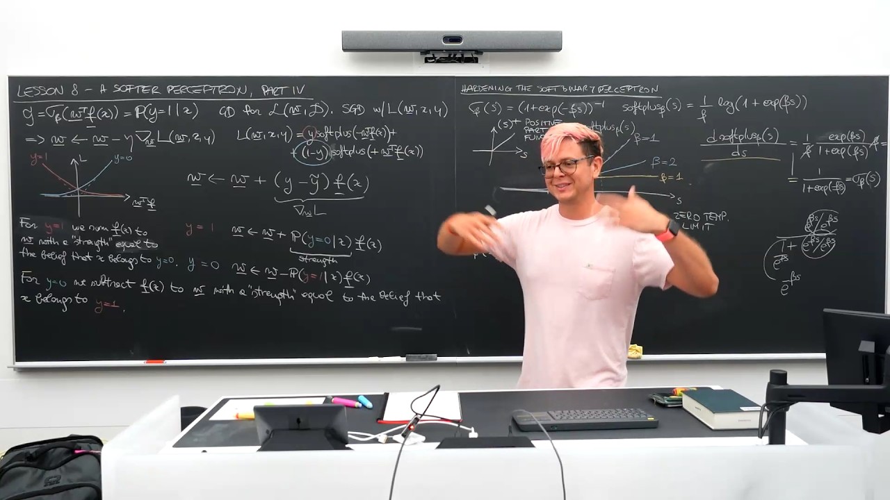
Lesson 08 – A softer perceptron, part IV: hardening and multi-class

the beginning of the lesson I'd like to share a few words about what I'm trying to do here. Right? So the content we are covering here is not really important. I don't care what I'm teaching like the things we are teaching yes somehow are relevant depends what relevant to what are they useful no why am I teaching this right this is just a arbitrary topic I'm using for teaching you a language what language you're pretty aware languages have words and then there is some sort of grammar that is telling you how to use this word to make statements in our case the language boring is the language of math and perhaps somehow physics physics and then we are trying to put together sentences by applying specific rules. So the end of the last lesson which what did we do in the last 15 minutes on the last class >> I just do >> what what what exactly yes we and that's the final title but what did we do like what did I write on the black >> partial derivatives >> partial derivatives right was there any teaching going on in that part no right because we were applying the same procedural knowledge that we already acquired from mathematics to just get a specific point to a specific result. So we started somewhere right we wanted to figure out how to perform what was the topic of last lesson >> gradient descent for the specific case when we are dealing with a specific loss which was equal a specific cost which the name of this cost was >> almost there's a there is an adjective for that cross entropy binary cross entropy right so we wanted to try to compute the gradients of a binary micro entropy. Why? Because that's what is going to allow us to figure out the optimal weights. What are the optimal weights? >> The minimum loss. Remember what is the connection between the loss and the where did we come up with the loss? Like how did we come up with the loss? >> Average percent loss again. >> Average percent loss. >> Yeah. Yeah. Yeah. But where it comes from, right? We started from some >> point. Yeah, but I know sh that loss when we are minimizing that loss we are doing something else right that loss the loss is something we like to to use but the loss comes from somewhere right you have to be very sure you're not you can reproduce those what's it the likelihood right remember we were talking about the likelihood when then we introduce the low likelihood and we start we don't like negative numbers so we talk about the negative lo like and therefore the weights that are minimizing my loss are the same weights that are going to P >> finish my sentence. Come on. >> Increase the likelihood like increase the likelihood. >> Not increase but even more. Maximize the likelihood. Very good. Right. So that was our objective. Then we just apply some rules from math and so that's why I didn't explain that's I just went through and then eventually I wrote a final statement but then we just said okay we are five minutes after class. We didn't understand perhaps the meaning right? So we did apply some grammar rules to get somewhere. We we arrived. We don't know where we are more or less. That's how we finish previous class. Uh so I just push it. I know there was no understanding but at least we got somewhere. Now let's figure out where we arrive. Okay, that's pretty much the first part I wanted to tell you. Moreover, in the first quiz, I only test you on words. It was completely superficial knowledge whether you actually checked you go through the notes or not. That was first quiz. On the second quiz, we're going to be actually starting to use some of the grammar we introduced, which is the grammar from mathematics to put together a few things to get somewhere else. I don't it's not going to be too hard, but it's going to be you have to make sure you understand what we have done. If you just memorize everything, you cannot answer this question because you have to apply the same grammar to something you haven't seen yet, right? So you have to be able to reason. So if you if something doesn't make sense, that's when you have to reach out either to me if you prefer or the tutor or the course assistant. This stuff makes no sense. Cool. Let's figure out why, right? Where did I fail in my explanation? So if things make sense, then you can actually tackle any other problem outside this class. That's the whole point. Whenever I get students in my graduate course, they can't reason. Oh, okay. My own students, the one I do research with, they feel they are a bit shy because they don't know they can step in the word without having someone that is next to them. Right? At the beginning of the last class, I love that someone came up here and asked me a question. Yes, I'm here for helping you. But then you have to be becoming independent. By the time you finish this course, you should be feel confident enough to oh, let me explore this part. What are my tools? Well, I have mathematics. I have a blackboard. I have some functional brain hopefully. And then let me try to reason through. Why do I put you I think you remind me. I forgot some bars underneath the W, right? Was it you? Okay. Why do I care about the bar underneath W? Oh, the vectors, right? >> Also, there's a difference between the vector with the arrow on top and the bar underneath, but doesn't matter for now. Why do I care about the bar? >> So, it's a vector. But why do I care about the fact that you know that that is a vector >> because it has different properties than the scalar >> there there is meaning right each symbol I draw here there is a symbolic representation which is how language works with different symbol but then behind the symbol that is like a placeholder there is the meaning which is the object that stays connected to that symbolic language. So we use a symbolic language to communicate but then underneath we actually are connecting making a onetoone connection to the real things. This actually comes from logics logic and the I think this is called a real realization if I'm not mistaken. If you don't know what I'm talking about it's okay doesn't matter. But the point is that I'm using I'm trying to teach you a language. We could be teaching I could be teaching you dancing cooking Chinese whatever doesn't matter. The point is that we are becoming trying to become fluent in this uh language. That's the objective of the course. The content is not really important. You should be able to how do you learn a language? Okay, there you go. >> Speaking. >> Speaking, right? If you don't speak and you just study the grammar book, can you say something? [snorts] You had to speak. It made mistakes. someone's going to be correcting you, right? And then that's how you learn how to communicate. If you can't speak, you have to make mistakes. That's why in this class, I very encourage you to make mistakes such that we get comfortable in using this language. Okay, that's the whole point. Done. Moving forward to today's topic. Again, every time you get you don't know what's happening, stop me so we can get back on track. We start with the recap of the last lesson because I said we did a lot of steps. We arrived somewhere. We have no idea where we arrived. So, so let let me let me explain to you where we got. So, lesson lesson number eight, I believe. Guess what's the title? It's soft after part four. We're going to be adding a title in a second. I will not put the title for now. We're going to find out what we talk about by the end of the lesson. We were talking about the softer binary perception. Remember that's the only thing we have talked so far. So we were we said that our prediction y t was computed by applying this sigmoid to my inner product between the weight and my feature vector of the specific object. X is an object. these different vectors and then this was actually representing the degree of belongness to class one for my specific object. Okay. Yes, these are probabilities but you have to understand what is the mean, right? So I just use this weird uh expression. Then we talk about gradient descent. Gradient descent of what we were we wanted to do gradient descent for my curly loss which is a function of my weight. Right? tells me how bad my graphs are for a specific data set. We decided to actually do SGD stoastic descent by minimizing the per sample loss which is the badness of the weight for the specific x and y pair. Sweet. How do we come up with gradient descent? We we're talking about going on a surface, right? We are on a surface and on whatever dimensional space. How do I know if the surface goes down or goes up? Up or down? I have a specific tool which is called the >> no >> I am at this point I'd like to know is this direction going up or going down >> directional >> derivative in this direction I know this stuff goes straight meaning what direction is this if the thing is like this directional derivative is zero this means I am moving along >> level curve >> a level curve right it stays flat like I'm just moving on the same thing and then instead I find a different direction and then you know I'm going down means meaning that that direction is going to be described by this scalar right the direction derivative is a scalar value in this case is negative right I went downhill instead if I find another one I go up means the direction of derivative is a positive number so that's going to be telling you the slope of the thing you're walking on right sweet so we found out that if I find if I turn around, I can find a specific direction which has the steepest descent. Amazing. I like to go in that direction to minimize this average loss by doing it one sample at a time. I pick one sample, I do one step down. I pick a different sample, it's going to have a different loss because I have a different sample, right? This is the average of all of these. This each of them are going to be different for every sample I pick because every sample is going to have a different feature. Right? So every every sample will have is going to give me a different overall value and then I just figure out for that sample where is the low like the steepest direction which is not necessarily the same as for this guy right somehow it's noisy anos approximation. Cool. So we said that stoastic in descent we are doing what? We are updating our W which is our current location. It becomes the previous W. Then what? We choose the direction of steepest descent which is the negative direction of the steepest ascent. Right? So we're going to be subtracting whatever scalar number between 0 and one whatever scalar number a positive scaling factor which is called learning rate but we don't care we can set it to one gradient with of my per sample loss with respect to the weight and this is going to be for my x wx and y okay think it's correct yes so step by step we go downhill sweet we apply this to my laws For the softer perceptron, for the softer perceptron, we have that L, W, X, and Y is going to be, let me just write the final formulation. I think you are familiar with this one. Soft plus of the negative thingy and then plus one minus Y soft all these, right? All right. Question. >> So assume we're only distributed. >> Correct. Correct. But we don't care. We're not talking about probability. We are cyberneticists. Relay statistics and probability to the different department. But yes, that is correct. We assume a Bernoli distribution on the on the flipping of the coin. But it's a conditional Bernoli because you are looking at the specific X, right? So it's a conditional probability. It's not just blindly flipping the same coin. You look at the email, then you try to estimate the probability. Yeah, >> I missed a bracket. Thank you so much. Right. I care about those things. Although Yan mocks me so many times. You're going to go crazy when I do. Okay, never mind. Once again, the same drawing I drew last time. Oh, I'm drawing things. I'm expected you to be able to draw. If I ask you draw this and I haven't drawn it before, you should be able to know how to move your hand in a drawing fashion. Right? All right. On the horizontal axis, I'm going to put my inner product. Okay. On the vertical axis, I will have my loss. We have two faces. We like to use the red for this one here. We like to use the blue for this guy here. Right? And so for the let's start from the blue one. What is the uh shape of the soft glass with a property thingy? It's going to be a 45 thingy here. It's going to be zero over here and it crosses at 07. So this stuff goes down and it goes something like that. And this is for my y = 0. And then for the other one, same down here, down there, it comes down and it goes like that. Right? This is for y equal one. Okay, just one more time. We just did that last time. What does the blue curve tell you? If my label is zero, I will pay a cost for positive inner product. So this thing here will try to get me. I mean if I if I move to the left hand side I will pay less. Who's moving to the left to the right here? To the left to the left there away. But who's moving the weights? >> You're in the center. Right. So if you are choosing this we are going to be moving to the left. Why is the case? So let's let's say I'm here. What is the gradient of this thing? One. Negative or positive? >> Positive. So if I'm going to be stepping towards a negative value, >> why to the left? >> Reduces the loss. >> All right. Well, >> what is this thing here? This is the inner product. >> Now I I replace W with what? >> Smaller. >> Smaller W. Therefore, the inner product if I didn't change F will be smaller. You can see this. So this expression here moves me to the left if I am on the right hand side with a blue class. If I over here the derivative is very tiny. So I will not be moved much. On the other side if I am on this left hand side and I'm at the class plus class plus class plus class plus class plus class plus class plus one I will have I will incur in a large cost in a large loss. If I compute the derivative at this point is a positive number a negative numberative. is a negative number. Therefore, I'm going to be subtracting a negative number. I will increase my W. Therefore, the inner product with respect to the previous one, if I have now a larger a more a lesser negative, right? W or like a larger W in in I will move to the right hand side. Right? So, this is what pushes me to the left to the right to pay less this expression here. But then we actually did write the functional expression. And so what was the functional expression when I compute the partial derivative when I compute the gradient of this loss? Remember that was the final part which is so remarkably confusing. Why is that? Right? So we had that my if I actually we didn't compute that on the last part. We wrote that my w is current w plus yus y* f of x. Right. And unfortunately, well, unfortunately for you because you're going to get confused. This is exactly appearing as what we have seen this before. This used to be our >> binary perceptron training wait update. >> Yes. Whatever he said the update for from who who's the guy who come up with this stuff? >> Weber. >> No. Uh >> blood when? >> 57. >> Yes. Okay. Amazing. You're you're a good parent. >> All right. >> Why is this completely different? >> Because not binary binary. >> Exactly. Whatever you said. So this thing here, it's a number between 0 and one, right? Therefore, this item here is always a number between negative 1 to + one. Okay? So, before we were either making a mistake or we were correct. Now, it's no longer the case. Now, there is a degree of wrongness. Right? The further you are on the right hand side, the for the blue class, the more wrong you are. Will you ever be right? Will you ever have zero here? >> No. >> No. So we always make a mistake. Oh ouch. Remember we were talking about the fact that the perceptron was able to converge if the data was linearly separable. Can we converge with this thing? No. Why? We obviously going to be wrong unless >> we have a decreasing learning rate. >> No, there's no learning rate right now. This is the actual gradient, right? This is my this is the grade. Unless we allow a bound for the >> Yeah, we are not allowing any bound, right? So, >> Android GPS. >> No, sure. The point here, this thing here, this is logistic regression or logistic classification, I prefer to call it, will never stop pushing weights because this stuff never goes to zero. Right. That's an important part, right? Yes. Right. Okay. So, Oh, yeah. So let let's actually have a few the two options. So what happens with y equ= one with y = 1 we are I just rewrite this thing we're going to have w plus 1 minus probability of one which is probability of zero. Right? So this is probability of y = 0 or my x times my official vector. Okay. So my y the true target is the plus one. But then my output right my my probability for one can never reach one. Right? It's going to be always a little bit less than one possibly. And so I want to make the inner product larger. So I will still sum my feature vector to my weight proportional to how much I still think that X belongs to the other class. Right? If I would be 100% sure that X belongs to the one class, how much is this probability? >> Zero. >> Zero. So I I would be stop I would stop. But this stuff never goes to zero unfortunately. It's going to be always a little bit something, right? But anyway, at the beginning, let's say I'm 50/50, I don't know. So if I'm 50/50 for blue class, red class, what am I doing? I just sum one half of my feature. The more confident I become with the fact that this specific X belongs to the red class and I will sum less and less feature for that specific X to my Wait, fine. >> You don't understand. Are you understanding? Okay, maybe you're just asleep sleepy. Who's not understanding this part? You. Okay, I try again. This one here works so far. >> Yes. >> Okay, I just decide y equal one. So this is going to be one minus the probability of the red class. >> Yes. >> Which is probability of the blue class. >> Yes. >> Okay. The f is the same as f here. >> Okay. Did you understand everything now? Yes. >> Okay. Great. Other people getting confused? Okay, one more recommendation for the one of you that are not taking notes. If you don't take notes, it's very it's harder for you to actually figure out what's going on, right? I'm writing things on the board because I think maybe everyone is taking notes. No, you're not taking notes. The the thing is that I could show slides, right? And then I just whatever. Instead, I do all this kind of standup comedy because I hope it's going to be more sticking with you, right? But then if you don't do the exercise of writing down, then it doesn't stick, right? Anyway, so far great. Let's see what happens with the other case, right? Go ahead to write the English. Maybe write a thread in English or i= 1 sum s uh with a multiplier with a strength proportional right to the belief that x belongs to the other class, right? All right. The other the other case is going to be similar for y= 0. We're going to have that my wal this is zero. This is minus the probability of the correct class. So minus probability of the red class time F. In this case, I just do the opposite. So my prediction should have been telling me this is a blue blue guy, but maybe I'm not 100% confident with that, right? And so maybe my inner product is still somehow positive. So how can I make my inner product more negative? I subtract my feature vector. how much for the same amount that I believe that that X belongs to the opponent class right so if I just a little bit think it belongs to the other one then I just subtract a little bit if I believe it's very very belonging to the class the red class and I subtract a lot that specific feature right so we subtract with a strength that is given to us by the belief that that X belongs to the opponent opposite class This is the meaning of this expression here. And so here for y = 0 for y equals 0 we would like to have negative inner product. Right? You can see here we'd like to have negative but it's not completely negative or it's not negative enough because every point here you have you will pay a cost right you will never you pay zero cost only if you go completely to the left right. Which one are you talking about? >> This is a proportional to the >> Yeah. So this is my Okay. This is my with a strength equal to There you go. Thank you. That's better. With a strength equal to [clears throat] better is correct now. So we are summing this case with this strength, right? This is my strength which can go between zero and one. Zero I am weak. Don't push one is like full full strength. Okay. Or the other case. So for the y equals z we subtract the feature w right with a strength equal to to the degree of belongness right to the belief to that x belongs to the So this is the semantics the the meaning of the result that we got last episode. So moving forward I like to bridge back from where we came from. So since this equation here reminds us so much of the previous guide that you mentioned before, let's get back there. Right? So how we do that? Let's harden the soften perception. Right? So hardening the soft binary perception. The thing I like is the freezing. Right? So the the analogy we are talking about why we talking about freezing frozen frozen >> molecules moving >> yeah but it's coming from our who's controlling the the temperature here >> the beta [clears throat] coldness >> beta right beta is our coldness so we're going to be playing a little bit with beta how many soft things have we seen so far >> where not in my class in our class right we cannot Use words we haven't seen in this class because you're cheating. What soft stuff we have seen in this class? >> Soft plus is soft in the word right. So very good. >> But before that we actually soften this thing here right at the beginning of the of the thing. So we were talking about the softer softer W right. Who's this guy? So this is my softer sigmoid that we I think yes we already seen it right? If I change the the temperature I can make it a more rigid sigmoid or a softer thing. How do you harden a soft term ice cream in the freezer? How do you melt the ice cream? >> You warm it up. So how do we freeze this sigmoid here? >> You increase the the the beta. Okay. All right. So, but then we actually are bringing in the new guy here which is going to be the soft plus beta and I haven't show it show it to you and I just write it down. I'm going to be explaining a bit why it's like that. Okay, this is going to be my soft class with the parametric inside. Okay. So, let's have a look at this guy, right? I'm going to use for at the beginning and let's call it right here soft soft. I think there is a web based graphic calculator. You can add parametric uh span, right? I I should maybe I can put the link on the on the on the Google doc at the end. Okay. So how does it work for beta equal one? We already know we have the 45 guy here. This one goes straight down here. We cross at let's say this is going to be one. Uh 07 is going to be something like this. So we come down this way and this is our soft class for beta equal one. question. I will use the blue to show that it's cooler. How is going to be going the soft plus with twice twice as cold plus >> how do you expect this stuff to to to change or >> we just take another bis sector between that. >> Okay. He's going he's going for the bis sector. How about other people? >> Ah no it was proceeding >> the synthetic behavior is the same. Why is the synthetic behavior the same and how you prove it? >> So for instance as uh s goes to infinity uh the one becomes irrelevant. So it's exponential ps when we [clears throat] take the logarithm it just becomes ps over b. So it's s the same as the normal uh soft and that is goes to minus infinity. It's the same it's zero. the next 15 minutes of class. Yes, I think you're in the wrong class. But yes, no, everything is correct. You're just ahead, like one 15 minutes ahead. Great. Good job. Are you math major? Math minor, but minor. Okay. Sure. All right. So, let's see what he just said. Did you hear what he said? No. Doesn't matter. Okay. Sure. So, we are going to be looking at this thing on the right hand side. He was claiming that this stuff goes at different speed. He's like, "No." So, let's see who's right. But I think you already figured. So let's compute here the derivative right of the soft plus beta s in s right derivative of this thing here is going to be 1 / beta 1 over this stuff over here 1 + x beta x time the stuff inside right 1 + hold on the derivative of the stuff inside right this one is the only one surviving X beta X times not don't answer time >> beta right there there's one more thing falling down okay so beta goes away with beta I divide by the exponential so I get 1 / 1 + x of beta ses beta surplus of minus beta Almost. You're saying the almost correct the sigmoid, right? He meant the sigmoid sigmo. You actually tricked me. >> S, right? >> All right. Sigma though. Yes. >> I'm a bit confused. You have the exponent of BS over 1 plus the exponent of BDS and that equals 1 over 1 plus the exponent of BS. >> Correct. Right. So BS is not BS. That's This is beta s. Right. So I I divide by the exponent at numerator and denominator. So this one becomes one. This one becomes one. This one becomes exponent of negative beta s. >> Okay. >> Do you see? No, you can say I don't see. >> Yeah, I don't fully see. >> Okay. X is E to the right. So this is written E to the beta. >> Yeah. S divided by 1 + E to the beta S. I divide by E beta S. So I have this one divided by E beta S. This one divided by E beta S. This one divided by E beta S so far. Okay. This one is one. This is one. This is E to the negative E. Oh, there's a negative before the >> there is a negative. Yes, that's that's there's a negative in front of the beta. That's why this is a sigmoid. Okay. Yeah. >> If there was no negative, that would have been >> sigmoid of the negative, right? >> Okay. So, how does this look? Right. What color do you want? Orange. I decided for you. We don't don't like colors. Okay. Cool. So, let's hand the derivative. Where? here. How does the derivative look? So from here onward, can you guess how much is the derivative like from here to the right side? >> One. >> One, right? It's it's Yeah. Very good. So if this is my one, it's going to be something like that, right? It's going to be symmetric. From here, I had derivative is going to be here. Here the left zero. >> Zero. Right. Of course. And then in the middle is going to be crossing at where child >> one half. Yes. So it's going to be going here. So it's going to be something like Yeah. Okay. Sweet. Okay. So what happens now for beta= 2? This is beta equal one, right? What happens for beta equal 2 with a sigmoid? What's a yes? What is a frozen sigmoid? >> Sharper. >> Sharper. Right. So the other one is going to be still one, but it's going to be crossing where? Twice as fast, like twice as early. Right. So the other one is going to be crossing here like it sticks until here to one. It sticks until here to zero and then it's going to be going faster. Right? This is for beta. Right? Therefore, if I'm going to be drawing my cooler soft is going to be exactly as this one here, right? The derity is one. So, this is 45° until something here. Where do we cross? Okay. And where do we cross the the vertical axis? >> Big sigma pals 2. >> Which color is this? >> 0.7. [clears throat] >> Okay. Now first think you green shirt. >> Yeah. Where is the soft plus with beta B beta equal to going to cross the vertical axis? 0 >> 0.7 over two >> 0.35. How do you answer this question? [clears throat] >> Because we said that >> okay where do we cross the vertical axis? How do you find out the crossing point? You can say I don't know. I can tell you. Don't worry. Okay. What is S value at the vertical axis here? >> Zero. >> Zero. Very good. So, just put zero inside here. How much you get? >> Say again. >> Log of one. >> Log of one. No, instead for the s you put a zero too. >> This is s, right? SO it becomes log >> two >> / >> which is >> log two >> two. So it's log two divided by two >> is it good? Okay. How much is log 2? 07. How much is log 2 / 2? 7id.35. Right. Whatever. And so it's going to be half the height of my other crossing. And so we come down here. same way and like that. Okay, this is for my bet theta equality. So if I keep freezing, if I keep increasing beta, what happens here? What is the behavior? The synthic behavior, >> it's going to approach zero, right? It's going to be going down to like going down to this thing. What is the actual if I if I write it down here? >> But this is a deep learning word. We are not yet talking about deep learning. We are doing math. Yes, the answer is correct. But we have a different name for this function. >> What's the name of this function here? >> Let me say >> positive part. >> The plus function. You seen the plus function before? >> What? >> The plus function. No, because it has different name. So this one is going to be written like this and it is called the positive positive part function. Okay. So this is the positive part function. What is the positive part function? If a number is positive, the positive part just returns the same number. If a number is negative, the positive part is returning zero. Okay, if you haven't seen this uh Wikipedia, I will add the link to the Google doc. We'll use this a lot in the next part of the course, but so far you can just tell me that the soft plus will converge to the plus function. So we have that soft plus soft plus beta x converges for beta that goes to plus infinity to the positive part and we had that the sigmoid beta of s converges for beta that goes to infinity. We already seen this several times. Either you can write x larger than zero or which is going to be the same as the heavy side fun. This is not the cross entropy is the heavy side. Okay, we already seen the second part. We haven't seen the first one. And how do we call beta that goes to plus infinity this is called the yeah this is the zero pressure from physics but sure. zero kelvin of course I mean are there other degrees questions question one question two >> like for the quizzes only I'm asking like are we supposed to know how to derive this like how to prove this >> everything that we have seen so far you should be able to produce then I'm not necessarily going to ask you those things. But for the final exam like when I when we have like the >> the oral like you are supposed to be delivering any of these classes part right I can ask you we start here how do you go there you should be able to the point is that you should be able you're fluent in reasoning yeah >> I to know like to derive something that's outside the class like you didn't do it >> so here I'm showing you what is the procedure to go from point A to point B given that you have the words and you know the objective I could provide different words different objective and you have to apply the same structure right so it could be that you just have to use the same language it's not going to be like the the words might be different the object the target is going to be different but then the procedure is going to be exactly the same as long as you can just put together those words yeah right so even though there will not be meaning So in those classes, you might not know what you're doing. Doesn't matter. You can just trust the the process that you already know how to walk. You're walking on a new terrain. Just keep walking. Like don't don't wander. Don't don't don't ask yourself where I am. That doesn't matter. Just just keep walking. Right? So I'm trying to teach you how to walk such that you're feeling comfortable in walking yourself. But yeah, it's not if I do it's not going to be too crazy. Just same same thing we we doing here >> same level >> same yeah [laughter] you have taken calculus one right >> and then two >> yeah yeah yeah so I will there is a question that I asked five times and we'll for require some mathematical concept that we have not touched in this class but you should be able to use it but it comes from previous classes, right? That's just one question I had, but it's cute. I don't know. Usually they they everyone managed to to to answer the question correctly at the final exam, but they were like, "Oh, we we have to use that." Yes, you have to use that. So, you usually know what you have to use, but you were like surprised because we never used it before in this class. Don't worry. Done. Okay. Next topic. Picture. doesn't how do we call the title so far? So we can call it uh harder software perceptor. >> Yeah, but it's not finished. So second topic, right? So we have two titles. We're going to have two parts. So we're going to be going back to our friend M class. So where we where were we? Where where were we last time? Like back in the multiclass case, we were dealing with multiple classes, right? So we have K classes, right? We have we have capital K classes K one two capital K. Then how were we making the prediction? So what do I need? Also since I have capital K classes therefore I have capital yeah capital K. So we have capital K gases capital K weights. Uh therefore we also have capital K inner product or my uh X. So how are we performing inference? My output from my model is no longer called Y tilda but we change the notation. We call it Y hat, right? Why is Yhat hat hot hat? Ar max >> because this is the arg right. So y hat is the arg max over all possible case of those inner inner products and then how we were performing learning. So if my y hot is the same as my y don't do don't don't do anything right don't touch it it it works it's making no no errors otherwise we're going to be using a error correcting mechanism meaning you made an error so we fix it so for the case where my prediction is not matching the reality we have to do two things so this means that so if yhat is not Y it means that W Yhat transpose F is larger right then W Y transpose F correct right I have if if it's incorrect meaning the largest inner product is not the correct inner product so in this case what we have to do if this is too large we have make it smaller. If it's too small, we have to make it amazing. Okay, so we are going to be doing lowering this guy here. So I take my the weight for y hot and I update it as the weight for y hot minus right my feature vector for that specific x and in the other case is too tiny. So my W for the correct class instead I want to make it larger and this is like recap from last time but guess what we're going to be introducing now some new notation and just so today today well this part is going to be me introducing new words understanding is the same understanding as we have so far I just change notation why well you're going to find out very soon how many of these things I have capital Okay. Can I compute them all together? Yeah. So, we can compute all K inner products at once, right? With what is this stuff? Right. So I have to do capital K inner product. How do I do multiple inner product product at once? I stack all those transpose weights. Right? So here I have my first W and I have my last. So I have just a stack of rows. If I have a stack of rows and I multiply by the single vector, I'm going to be getting a stack of scalar values, right? Is a stack of inner products. S that's already here. [snorts] S is going to be S1 S2 S >> and S1 [clears throat] is W1 T multiply by F. All right. Okay. So, let's define here Y bar. Oh, something new here. Y bar is going to be the one hot of my Y. So for example let's assume that y is equal four and then capital k equals say six. Therefore I will have that y bar is going to be 0 0 0 one zero. So one hot is a vector of all zeros where the index corresponding to the number inside the parenthesis here is set to one. Right? It's one element hot. Hot comes from electronics meaning there is a voltage there but I belong here. So this allows me to convert a integer into a indicator function. And in this specific case I have one additional information which is what is the total possible indicators I have in this case it's so given that this uh we introduce this new notation can I rewrite this stuff here in one go? Yes. So we can actually write a more compact update rule in the following way. a more compact more compact modified date rule therefore can be written as and now let's see if I it up so I have my big set of rows is going to be the big set of rows plus y minus Why? Why can we do that? Do you understand? You can see on the there, right? If you cannot see through the B. So, let's figure out a little bit what this thing is, right? Do we understand what this right hand side is? We haven't seen this so far in this class. So far when there was this T the transpose we used to talk about >> in product >> inner products. What is the thing written on the board today? >> Outer product. >> It's the outer product. Right? So let's let's see how it looks. Right? For example, let's assume y = 4 yhat = 6. Therefore I have y minus l hat is going to be what? Can you tell me? >> 0 0 0 1 0 1 >> Yes I will write it here. 0 0 1 0 minus one. Okay. This is a column vector. If I take this guy and then I have my f transpose. So what is franspose? That's my feature down right. So if I multiply those two things together, let me actually write it properly. So I have 0 0 1 0 - one times f_sub_1 f_sub_2 how many? We don't have six because it's K. >> Oh, no. It's the same F. No, >> we haven't specified it. >> We don't. F has the number of features, but we know that the same amount of features as the R weights. So, it should be K + one. >> No, K minus one. K minus one. No, should be K. But that doesn't include the bias, I think. I don't know. We don't we don't know it. So we don't know. We don't know. I mean that the answer is we don't know. That's the correct answer. What is going to be my f right? I have n features. If we have the bias, we also have the additional plus one at the beginning. But whatever bias, right? And so if I multiply these two things together, what do I get? >> What do I get? >> All size * n, right? So I have this thing here is going to be first row. What is the first row? >> Zero. Okay. First row, second row. Okay. This is becoming confusing. >> F12. >> Yeah. Then >> and then >> any stuff lives where? Aran. Therefore, this guy also was leaving where dark and so I take my matrix. Then I this guy over here. I will therefore sum my feature vector for the correct class weight. Right? Associated and we sum to the weight associated to the correct class. I will subtract the feature vector to the weight associated to the most offending class. Why do I call it the most offending class? Because it's the class that has the largest energy in a product. Wow, we have so much more time. So, I didn't know we were going this far. Maybe. Yes, I knew. So, questions. No questions. Right? This is just notation. Why did I do this? Because now allows me to just introduce a single four characters to bring in a whole new topic which requires four characters. Guess what is the new topic? >> Yes. No. >> Yes. I don't know what they're softer softer [laughter] softer multi- glass perception right remember perception is the hard our hard thing then we are talking about this softer thingy that is connected to the probabilistic real and so on okay so let let's bring back the the softer well the [clears throat] whatever we did with the binary case. So instead >> this was a hard percept multiclass perceptant because it got k1 to whole numbers like y why y hat it can only be a whole number that's a hard multiclass per se and now we're going to the ones where they could be any floating point >> almost do you find out soon so instead of using a hard decision boundary we introduced a degree of belongness. So which degree of belongness we have seen before right. So for the binary perception we talk about talk Okay, we talk about this thing here. Be careful. I don't have the equality inside. So, what is this item over here? Remember, there's a important distinction between this guy here and the other one which has a y equals something, right? There are two different things. What is this guy? This is probability of y. Sure. [laughter] What is the difference between this one and the other one where I write y equals something? >> That is probability of x belonging to the class of y. >> No probability but but y is one. >> Okay. So that is probability of y being a specific class. This is the probability of >> of all possible classes. Right? >> Very good. >> So I will write it this way. You should be able to write it the other way. I cannot say more than this because I I yeah this is sigmoid of wf x for y = 1 and then it's going to be sigmoid of negative wf x y = 0 and here we are using basically v sigmoid to convert what is this up side. [snorts] We use a sigmoid to convert my linear sum, right? The real number into yeah into something, right? We're changing the interval. We were going from a real number to something that is limited between zero and one and this flip brackets means that there are no open open side but we don't care. So now what's happening for the multiclass for the multiclass we have capital K inner product SK which are we are numbers. How do we convert those things into numbers between zero and one? So we're going to write here the following. So in this case we're going to have the y bar underneath which is going to be and this is coming from something that we call soft what what is called that one. So this is of r max of what is this thing here. So this is going to be equal to x of so this is my x right. So this is exponential of s / k = 1 to calculate k of exponential of s k. This thing here at the numerator is going to be the vector of e to the s1 e to the s_ub_2 e to the s capital k transpose. Right? So the numerator is going to be the vector where I take the exponential of each component and I divide by the sum of all the exponentiated components. This function here in this course is called the soft arc max. Why? Next episode I explain to you. The whole point of this class or the second part of this class was that we go from whatever we seen so far with the arc max to something that is the soft arc max. Next episode we going to try to understand what is the relationship between this soft arc max and the other arc max. And we will probably introduce a R max that operates on a on vector >> question. Yes. >> Like cuz we have like a range of okay for the binary class why we don't have the range of >> oh so this is going to be a vector. >> This is a arm max of a scalar. If I write okay there is one more line here I will write it here I just write here I think it is just a small thing if I do the arc max of a vector is going to be one of the arc max for the k of x k okay so the arc max of a vector is going to be the one arm max of the scaler So one hot user >> the one hot allows me to convert integer into a one in the vector right and so whenever we have the arm max of a vector I will use the 0 one the one output if I have a scalar it's going to be an integer I think I I missed I missed this one thank you for asking [laughter] what's the what's the triangle >> yeah that's a probabilistic simplex I can just write it here. This is the [clears throat] probabilistic simplex. >> You can check on Wikipedia. Doesn't matter. It's just a symbol. >> All right. Thank you for listening. Let me stop the recording. And these come