How promoters optimally encode transcription factor concentrations under time an physics constraints

from Lebanon from Beirut where he did the first studies up to masters where he moved to France. So he has been in a corporate technique doing the masters and we had a collaboration. So he's a longtime visitor collaborator. We published a nice paper last year. H so it's a good example of someone who comes from a field that is very different to his research field because you are an engineer. Uh so for him physics was all new when he came first time here and and also now he's doing biohysics which is also new for him so it's it's a good encouragement for all of you to jump to a new topic so he's a good example he can tell you many stories about it and now he's doing PhD with Alexandra Balchuk and Timura on decision making and other topics in biohysics which is the topic of your talk today so welcome. Thank you. Thank you. No, thank you so much for having me. I I spent some of the most beautiful months of my life here in Tieste uh working with Edgar and uh learning so much like on many different levels. This this place is extremely stimulating and I was super grateful to be here and very grateful to be be here again. Um okay, so let's jump into it. It's World War II. You are a fighter pilot belonging to one of the militaries of the world that own fighter jets. There are more and more these days. And you have been shot down over a city that you don't know. And you need to find the embassy of your country as fast as possible. And now the problem is you don't know where you are because you land somewhere. You don't have a map. You don't have a GPS and you land and you see this. So you see a street of uh in an unknown location and you see some people crossing and you try to tell yourself, okay, in most cities in the world, the population density is high roughly near the center and then it kind of slowly falls off as you get towards the countryside. So you try to substitute what you can observe for what you want to know. What you can observe is how many people are crossing the street and what you want to know is where you are to find out if it's worth camping uh on site or walking to the embassy. Uh so this is the decision you have to make and you're under pressure. You want to make it quickly. So what you're trying to do is you're trying to infer the location, your location relative to the center of town. You use concentration of people as an estimate for that and based on that you make decision. But actually it's worse than that because what you're really doing is you don't have access to the real concentration of people. That's a population average. What you have is a noisy variable. People crossing, people not crossing. And then you use that to do inference. And from that you say okay is the concentration of people roughly higher than this level or lower than this level. And then based on that you make a decision. So there's three parts to what you're doing. You're you're assuming that the information you're interested in is encoded a certain way a noisy way. You're doing the decoding yourself and based on that you make a decision. But jokes on you because I've been talking to you about developmental biology this whole time. So this is exactly it maps almost one to one to the way cells in the early part of the development of an embryo decide where they are and we were talking about that over lunch right uh recently it was discovered that you know you have different behavior when um an embryo is growing near the head of the embryo and near the tail of the embryo. And this reflects uh some of the earliest biochemical decisions that are being made on the way to developing the organism into a into a full uh full grown embryo. So the first decisions are for each cell. Oh, we're near the head, so we want to express this gene. We're near the tail. We're not going to express this gene. We're going to express another gene. So in certain organisms like the fly, this happens very, very fast. So flies go from one fertilized egg to a larvae in 24 hours. So that's many many decisions that have to happen in a noisy way because remember all of these are done um with molecules diffusing and binding to receptors and things like that. So there's a lot of noise and also under the constraints of well how well can you do this decoding in principle which is something we're going to talk about a lot. Also you assume that evolution has somehow selected for this process to happen efficiently because we observe it happening very fast and very reliably. You know like flies don't have a plus or minus 5% tolerance on where their wing is. It's very perfect almost perfectly in the same place every time. So somehow this information has to be encoded in a very faithful way. uh also there are constraints imposed by the physics of the problem and how things work at at molecular scales namely diffusion. We're going to talk a lot about that. It's going to be central to the talk. So the main question I want to talk to you about today is how would you design an optimal encoder? And in our case an encoder is a promoter which is just a piece of DNA. Here I'm symbolizing it with a black squiggly line. It's a piece of DNA that's located near the gene of of an organism and it's the region that's responsible for regulating the expression of this gene. So there's going to be some protein that floats around and binds to this promoter and based on that the promoter will activate transcription and transcription if you're familiar with it from high school. It's where uh an enzyme called RNA polymerase sticks to the DNA and starts to walk along the DNA and produces mRNA, messenger RNA. That messenger RNA gets translated into a protein and does things later. So this promoter is kind of the the the place where information about concentration is translated into another signal which is transcription. So it's the encoder. That's why I'm calling it an encoder. So um taking a step back and thinking about this problem of making decisions based on noisy data across time. So a very common situation that you encounter in life is something like this where you have something you see and you're trying to decide well okay is it a bird or is it a plane? So you wait a little bit and it gets closer and initially you thought it was a plane but actually it looks kind of more like a bird now but when it gets really close you know for sure it's a bird. Okay. So what you have been doing implicitly is calculating the probability ratio of these two hypotheses. So what you're saying is well I see something assuming it's a plane how likely is what I'm seeing uh compared to what how likely it would be if it was a bird and if that ratio is above one you say okay it's more probably a bird. If it's below one it's more probably a plane. Um the exact equivalent that you could be doing is taking the log of that. So this this thing now has to be below or above zero. Um, and if you actually put a threshold here, and then you' be very certain that it was a bird when your log ratio went above that threshold and then you would be very certain that it was a plane if it went below that threshold. 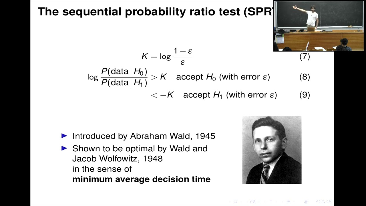So, it seems intuitive that you could do something like that. And actually, this was proposed uh by a guy called Abraham Wald in 1945. This exact procedure that I just described to you. You observe some data. You're trying to distinguish two hypotheses. You keep observing your data and you update a log likelihood ratio of the two hypotheses and when it goes above a certain threshold that you set in advance which is going to be related to the error that you're willing to make, right? Because you're going to make an error. You you know you don't always guarantee that you make the right decision. Everything is noisy here. So you fix your error level and you say with K log one minus your error over your error you accept and minus K you you reject symmetric hypothesis. So it was this procedure was shown to be the the decision-m strategy that gives you on average the shortest time to make a decision out of all possible strategies. So you could come up with other ways of trying to make this decision. On average this will be the fastest. Uh 1945 is not a coincidence. Yes. I >> have a question about the probability. What is the probability of the hypothesis given the data? Yes, that's a very good point and actually I've kind I'm uh I'm hiding something here which is that if you assume that you have prior beliefs on your hypothesis so without observing anything you don't have any reason to believe uh one hypothesis over the other. So you assume that your priors are equal 50% 50%. If you assume that then what you said is equivalent to this but you're absolutely right. the the way the the more correct way to do it would be to say what's the probability of the hypothesis given the data and that's called the posterior um but because right and I should have mentioned that because I'm assuming that you know a priori you you don't have a reason to prefer one over the other then these two ratios are interchangeable um right so this was um this was the result of research during the second world war so I I I I I I realized that my example from the beginning was which was not in inspired by by this fact but by some other facts. Anyway, so this is what it looks like uh visually kind of if you plot this log ratio and here I'm using a shorthand P of C to refer to P of data given C right and C here is the first hypothesis C plus delta C is another hypothesis that you know assuming your hypotheses are one-dimensional things are very close to the original hypothesis deferring only by factor delta. So this is what it looks like and your K threshold is horizontal line. When this random process crosses the line for the first time then you make a decision and this you can model it as a drift diffusion. There are properties that relate the drift to the diffusion and I'm not going to go into that. There's a lot of interesting work being done. So now I'm going to do a calibration uh question. So, I'd like you to raise your hand, please, if you if you agree with this statement. There's no tricks here. It's a It's calibration, so it's supposed to be very So, are there what 17 people? Okay, please, if you agree, raise your hand and don't be shy. So, okay. So, five out of 17 people didn't raise their hand. Good. Perfect. It's going to be interesting. So, I'm going to I'm going to run you through an applied example for SPRT. Now, so what I just did is I calibrated you. So, five So, 17 people, five didn't raise their hand. So, I'm gonna assume I'm gonna model you guys. Okay, you uh didn't raise your hand. This is the probability of new you not raising your hand. You could have raised your hand. You could have not raised your hand because you're shy, right? Times the probability that you're shy or you could have not raised your hand. No hand given that you're not shy. one minus the probability that you're that you're shy. So this is uh this is a very simple model of you your behavior that I'm going to use all all along the talk to kind of probe you and understand if you're ask if you're if if you're understanding what I'm saying or not. So the probability that you're shy we just calibrated it because we asked the question that is true and very obvious and everyone should know it. So you already know it, but you were shy. So you didn't answer. Um, so this is going to be the probability that you don't raise your hand given that you're shy is one, right? Because you're shy. So this is going to be P that you're shy. Plus this thing is the problem that I want to try to address in this talk that you didn't raise your hand and you're not shy. That means you're you're lost. I'm going to call this P lost. Okay. So uh P lost * 1 - P shy. Okay. >> Why is it lost and not disagreeing? >> Because everything I will tell you is is true. You cannot disagree. The only thing you can do is not understand because what I'm going to be testing you on is not uh trick questions. It's just going to be did you understand this? Can you explain it to someone? And I'm going to count on you to give me honest answers. I can't do better than that for now. So, um okay. Right. So now let's say okay what's the probability of observing K hands that were raised given that P lost my objective in this talk is to make sure P lost is above is below 0.5 okay so let's say P lost uh equals uh whatever P just going to call it P parameter maybe call it Q so that we don't get confused so this is going to be what? This is going to be K hands means I observe K hands raised. So k choose n p of no hand to the power n minus k 1 minus p no hand to the power k and p no hand we just got it here in terms of pshi which we calibrated and we got we got Five out of 17. So you're really shy actually. So what's that? That's That's about 0 28 or something approximately. 0.28. I Okay. I I I I ran my trials assuming it was going to be 0.1 or something, but that's okay. I think it'll still work out. So So what am I doing here? I'm writing down the likelihood of some data that I just observed based on a very simple and model that's very wrong also because there's many assumptions that aren't correct. But let's stick with it just to for the pedagogical example. So now if you want to do uh I want to write down the log likelihood ratio of p of observing k hands given that p lost um is equal to uh say 0.6 p of observing k hands given that p lost is equal to 0.4 four. Okay, now we can do that, right? You just take this, this factor cancels out. You're left with this. You substitute this value for it and what you get is something like uh correct me if I'm wrong cuz I did this yesterday evening so it might be wrong. So this is going to be n minus k log of Um, Pshai, I'm going to do this first. P shai plus p los 1 minus p shai um minus so p los going to be 0.6 here 0.6 six log of P sh. Sorry, my handwriting is not great on the blackboard plus K time log of 1 - P shus 0.6 Okay, so it's something like this. Okay, so I wrote a Python script to implement this and as the talk progresses, I'm going to ask you checkpoint questions and we're going to gather data and at the end we're going to draw the SPRT and we're going to figure out if you got something out of the talk or not. Okay, so the first checkpoint question is this. So if you have a data generating model, SPRT is the fastest procedure to make binary decisions on average. But you can come up with a deterministic scheme that can give you a faster decision some of the time for individual experiments. How many people agree with this statement or are comfortable or have understood this aspect? >> Yes, it's it's this. Sorry, I I didn't give you the the acronym, right? So, it's it's what this procedure is called. It's called sequential probability ratio test. Okay. So, it's a stochastic decision-making test. It depends on the randomness in your data. You can come up with a with a scheme that says I'm going to wait for 5 minutes and then decide if I have seen more evidence favoring H0, I will decide H0. If I if I find more evidence for H1, I'll decide H1. You can do that and you'll always decide in 5 minutes. If you do this because it's random, you could observe your data and you may, you know, take longer than five minutes sometimes, but on average um you'll decide in the fastest possible way. Are are you okay with this? I need to collect data. So raise your hands if you think this is clear. Okay. One, two, three, four, five, six, seven. Okay, that's that's I think that's good enough. Okay. So the I'm going to I'm going to do the thing here. So checkpoint number one checkpoint. Uh this is K seven. Good. Okay. Let's move on. So, SPRT was was uh suggested first as a general statistical test, but a few years back um it it it was applied to the problem that I described to you in at the beginning, which is uh biochemical sensing. So if you want to model the the very simplest um situation in in in biochemical sensing, you'll have one receptor and you'll have something floating in the medium around that receptor that can bind to it and that can unbind with it's a markoff process. So you can assume that binding times are exponential and the the time to arrive and bind is also exponential. The rates are going to be different. They're going to be governed by binding is going to be governed by C times some base binding rate. C being the concentration of the thing you have. Right? At high concentration, many things are going to arrive per unit time. So your rate is higher. The unbinding rate doesn't depend on C. When something is stuck, it just stays there for an exponential time. Then it detaches. Okay? So you can write down the likelihood. You observe. Okay. I look at my receptor bound unbound bound unbound and the durations of time. You use this data. You can write down a likelihood for this trajectory. It's very simple because uh you assume that binding and unbinding is independent. So your likelihood is just a product of exponentials. So you can write it down like this. You have um the probability of remaining for time s uh bound the probability of remaining for time t1 unbound and then for s2 bound and then you keep going and all of these terms ckb don't depend on the time so they collapse. This is just raised to the power n. N is the total number of binding unbinding things that that you observe. And in the exponential you get a sum. It's just a sum of the total. It's a total time spent bound total time spent unbound. Okay, this is pretty straightforward. You can take the log. The log splits nicely because it's a product becomes a sum. And then you say okay if you wait a long time you can approximate this as a drift diffusion as a brownian process actually uh with drift. So this is what uh CJ and Vergasola did in 2013. They computed uh analytically the drift of this log likelihood ratio. And what this tells you is remember SPRT is this uh decision- making process where you have uh you know you can go up or down etc and you decide when you go above K or below K and you have a drift on average if you wait a long time this is going to be governed by a certain bias in in your process and this drift tells you how good you are at making decisions uh per unit time. So if your drift was really high, you will reach this bound much quicker. So you can make decisions quickly and that means you're very effective at distinguishing uh your two hypotheses with each binding event. But if your drift was low, that means you observe things and you kind of can't tell if the concentration was high or low or whatever. So this quantity is important. This u it's going to be it's going to be important for the rest of the talk also to think about it. Okay. Um other people have uh done more things with this. They've done optimization of the rates. So far we've assumed so what I did here is I calibrated you with a simple question to understand what Pshi was and PI was an unknown uh parameter in my model. But what you can do is you can say evolution has access to uh you know evolution goes over a long time and you can say well assume a receptor has been optimized by nature to be very sensitive to concentration. What would this pshi be? This is this is going to be the essence of of my talk. This is going to be what I'm telling you about. So you plug in the notion that optimization can be happening here because these organisms are being selected to be sensitive to certain concentrations and we know that from from the the way gene regulation works. You know this protein codes for this gene and you have to know how much of this protein there is. So you assume evolution has done a good job and so you say okay we can optimize over this and you say so do you have an idea what py would be if we applied this logic here very easy question if I was assuming that you are very informative of your own level of understanding of what I'm telling you what should pi be it should be zero exactly so this is kind of the the the the the the trivial like sanity check. So um this has been also used in yes >> the average that you were taking earlier in the last >> over um >> over different traces right that's a good point so over you collect data over many trials or equivalently you can just wait a long time average over time average over experiments in this case is going to be the same. So this this same procedure has been used in stoastic thermodynamics very different context by uh some people in this room Edgar and collaborators to decide on if you observe a a stoastic process is it moving forward in time or backward in time in the same framework of uh sequential probability ratio you can use it and you can show that it has connections with thermodynamics that are very interesting. Okay. So now we forget about sequential uh hypothesis testing. Um I'm going to take you to another thread in in biohysics research that has been very influential which is a related question which is um so how sensitive is the estimator? If you if you think about statistical estimation uh and treat the receptor as a statistician they come up with an estimator how uh how much variance is there in this estimator the very old statistics uh framework. So another problem a common situation that people have in life is you you want to catch bus number six to go downtown and you you don't know the schedule and you see people waiting right everyone has faced this if you gone so should I run or not so you say okay let's say let's see the average number of people that that that I observe is is proportional to the rate of arrival of people but also the time since the last bus passed you can say that okay it's reasonable Then you could say, I want to try and use the number of people as an estimate for time. So it takes you, for example, three minutes to run to the bus stop. Uh you want to you want to find out as accurately as you can if if enough time has passed that it's not worth running because the bus is going to come really soon or if you still kind of have time to make a run for it. Uh I'm not encouraging you to do this. You should use the underground tunnel because it's very dangerous to run across the street here. Um but yeah so okay people arrive with a rate lambda uh the average number of people at time t is lambda t and you say I'm going to use the number of people so what you do is you invert this relationship average number of times lambda t you want an estimate for t you just take lambda and you put it uh in the denominator of the empirical observed number of people you don't have access to the average That's what you're trying to estimate. That's one way to make an estimate. It's okay. I suppose the number of people I observe is the average plus some fluctuations. So you take lambda, you put it in the denominator, and this gives you t hat, which is your est your noisy estimate of what time it is relative to when the last bus passed. Okay, you can say, okay, what's the variance of of my estimate? How good am I at telling the time using this very crude method? So you can compute it. It's one over t. So the more the longer you wait the lower your your variance will be and this is very typical for post processes you know uh this kind of uh variance that decreases so I'm I'm normalizing by t ^ squ here so uh 1 / t is very typical for diffusion processes and processes uh okay this is exactly what people did um in the 1970s to try and understand how effectively can a concentration Can can a concentration be estimated from binding and unbinding times? Uh so exactly the same method you assume that a receptor is making an estimate of concentration by counting the number of binding events and dividing them by KBT. So this is Chat BP uh because this is the estimator that was given by Bergen PCEL 1977. This is a very influential paper in biohysics. It kind of you know launched a whole series of investigations on how accurate can things be you know and you you include various elements correlation rebinding all kinds of interesting things that happen at the molecule level. So they came up with um just like CJ and Vasola. Oh okay sorry forget about what I said they they calculate just like just like I did on the previous slide the variance of this estimator. So how good do you do uh on average? And this is the variance. It's proportional to it's proportional to the inverse of A, which is the size of the receptor. If you have a larger receptor, you can get more statistics. D, which is the the diffusion coefficient of the molecule that's floating and binding to the receptor. If you have a lower diffusion coefficient, it's going to take longer for things to arrive. So that this hurts your your estimate. Also, uh the time, of course, if you wait for longer, you make a more accurate estimate. and one minus p is the probability of being bound. So that's that also has to do with the the properties of the receptor. So this is a very famous uh calculation. Now I'm going to show you a different way to do it which comes from a more recent paper uh a few years ago like 12 15 years ago now which is uh in the same spirit as as what I showed you before with with hypothesis testing. So you write down a likelihood. It's exactly the same likelihood as in CJ and VGA solo. You write down you see binding unbinding blah blah blah log likelihood. You get a term that depends on the total time spent unbound the total time spent bound plus these terms in the log. Then you say okay I'm going to take the derivative of this with with respect to C and I'm going to find the C that maximizes the likelihood of what I observe. So you do that and you get uh another estimator which is number of binding times divided by KB times TU the total time spent unbound and this is important remember I didn't show you I did actually here sorry there shouldn't be any brackets here I this is this is wrong it should be n the actual observed number of binding events divided by KBT t is the total time. This is if you observe counting if you do maximum likelihood you get n / kbt unbound. So what is this telling you? It's telling you that if you if you do maximum likelihood only the information contained in the times spent when the receptor was unbound. So when there was nothing these durations of time are those that are informative about concentration the duration of of time that uh something spends bound to the receptor doesn't depend on concentration remember and I showed you the the rates of the receptor one of them has C in it the other doesn't so this is showing up here showing you it's showing you that um if you wanted to extract the most information from your signal you should disregard the binding ing times only look at the unbinding time. So the inter arrival times and you calculate the variance of this and you get something very similar to Burke percell but now there's a four instead of a two. Yes. >> In a simple you are either unbound or bound. >> Yes. >> So the same information is total time or >> um Is that simple? >> That's true. But you don't assume that at time t uh the receptor knows exactly what time it is. I'm having time t here >> for the calculation. >> Okay. >> But this this is a good point. If you assume you know time exactly, then the two are equivalent. >> But the receptor doesn't know what time it is. So if they don't then you are adding one noisy thing that contains information which is the unbound unbound time and another term which doesn't contain information which is the the bound time here. Um okay so the total time spent vacant is what carries the information about concentration in this simple model. This is a checkpoint so I need I need to see some hands over here. How are we doing? Okay, thank you. Three, four. >> Yes, >> sure. >> The times that you in the previous slide are the sum of the unbounded times that we >> Yes. >> One unbounded and another is just for >> Yes. Think about the bus stop. If you observe the bus stop, you're trying to infer the concentration of people around. You observe it, no one comes, you conclude that there aren't many people. But if people stayed in the bus uh waiting for the bus for a long time, that doesn't tell you how many people there are. It just tells you that the bus is slow, right? That the bus is not arriving very quickly. So you get different information from different uh different observables. Okay, let's move on. So there's a lot of content. So let's see. So remember this guy um the log likelihood ratio for SPRT. Now I'm going to show you that these two things are actually two sides of the same coin. Sequential hypothesis testing on on the one hand. If you have this log likelihood ratio, you take the average over uh many realizations of your data and you take the limit as delta C goes to zero. So here I'm parameterizing the distance between hypothesis. So if you let your hypothesis be very close to each other and this is the regime where decisions are difficult like you want to distinguish two very close by levels of concentration with noisy data in that limit this quantity uh becomes equal to uh this thing over here which I'm going to call f and there's a result from the 1940s that tells you that in general if you have an estimate this is not an equality actually this is should be an an upper bound. Sorry, this should be an upper bound. The variance of any estimator is upper bounded by the inverse of this quantity. And now you see that these two things come from different ways of framing the problem. The first one comes from the the the framework of you have two hypotheses. You want to decide what they are. The other one there's no notion of hypothesis and there's no notion of decision. Even there is the notion of you want to infer something that you don't observe. You come up with an estimator. Your estimator is noisy. What's the variance of this estimator? No decision, no hypothesis, nothing. But these two are related via this quantity called Fisher information. Okay. Okay. You can breathe. Take a deep breath because there's going to be uh more more content to come. Okay. So, in the previous checkpoint, I didn't record, but there were I think four raised hands. So, that's okay. It's okay if it's slow because you're shy. Doesn't mean you're not getting it. That's how I I think about it. Okay. So, so this part was kind of the background. Um in our in our paper we we we talk a little bit about this Fisher information and the connection between these two approaches because many uh results in the literature on biochemical sensing in in in recent years have uh have either used one framework or the other. So we were just showing that you can just view them as the same the underlying the same thing. So, um, I'm going to be doing, uh, what we talked about, but with a slightly more complicated model of the receptor. I've been talking to you about a a receptor with two states, which can be bound or unbound. Now I'm going to show you a model that has four states which is a bit more realistic of how things actually work and which captures something uh interesting which is you can have u transcription factor which is the thing that you want to try to infer the concentration of and RNA polymerase which can be transcribing or not transcribing. So now the notion of bound and unbound is not the same as transcribing and not transcribing. There are four possibilities. You could either be unbound and I'm referring to bound refers to transcription factor bound specifically. Okay. So transcription factor can be unbound. It can be bound but you're not transcribing because you need many proteins to come together in order to initiate transcription. So you could be in an intermediate state where there's no transcription. You could be transcribing also without a transcription factor. This can happen. you know you can have RNA polymerase binding and starting to do your your uh messenger RNA etc or you can have both at the same time. So you have a model where you cycle randomly through these four states with certain transition rates. So these transition rates, the transition rate of binding just like in the other model is going to be proportional to concentration times a base binding rate. And you have all the other rates which are uh unbinding the rate of of binding RNA polymerase everything else in this four state markoff chain which are also limited uh by diffusion by by limited in speed. So these are two important uh things that I want to talk about which is you cannot bind infinitely fast. You're limited by diffusion. You can also not unbind infinitely fast. These constraints are a new ingredient that we're adding to uh this study and we're trying to do optimization over these rates assuming that evolution has chosen a model that's that's pretty good at doing uh at doing this inference problem but it's limited by the the constraints of the biohysics. So that's what that's what we're going to try to do. Uh I'll tell you a bit more about that. So it's okay if you're not not exactly it it'll be clear in a few slides. >> Yeah. >> About the third street that you're talking about. If you're not >> about the third street that you're talking >> Yeah. >> If you're not if there is no transcription factor but still you translating because of polymerase. >> Yeah. But that that protein loses the signal, right? It can be producing some other protein, but that routine you're not going to use for uh sensing that particular transmission, >> right? It it introduces noise. It's bad for you. >> Okay? >> It's bad for you if you're transcribing when nothing is bound. It's misleading because you might think, well, is it due to a transcription factor or not? I don't know. And that's a that's a essential feature of this model is that typically there are hidden variables. You can't observe your your mark of process completely. You will observe part of it and then what I'm going to show you is how well you can do given this. The the simplest example of a partial partially observed process. So your point is is a very good point actually. Okay. So you can look at two different observables. You can say well I can look at just like in Berg per cell you count the number of of uh transcripts. So before we were counting binding because binding and and transcription we were assuming that they were the same thing. Now we're separating the two. The observable we're interested in is transcription. So you observe transcription. You don't know what's happening with binding. Otherwise you're back to the two-state case. You assume you don't know that. You observe transcription. You count. Okay. And you see at time t uh which also you assume you don't know uh how many transcripts have we have we made another observable is you you look at the full history and you measure the statistics of transcribing not transcribing just like we were doing before and we ask what is the difference of using these two observables now with the partially observed process. So remember uh there's a direct relationship. What are we trying to do at the end? We're a cell. We're trying to figure out we're closer to the head of the embryo or the tail of the embryo. We want to decide uh where we are. Minimizing that decision time is the same as maximizing the fisher information rate of this comes from uh this relationship over here. So you minimize the decision time, you maximize the drift. Remember this was the drift. You make the drift larger. This drift is exactly the Fisher information. It's actually the rate. So it's time derivative of this is the drift. You want to make that as large as possible. So that's our objective right here. So we're going to do this. This is just another way to write the Fisher information rate F dot. Now because it's a time derivative of this thing what I showed you before, you can rewrite it as the second derivative of the likelihood of your observable either this one or that one. uh given concentration with respect to the log of concentration squared. It's a it's just some algebra to show that you can it's it's it's an approximation first order approximation to write it like this. Okay, we're going to do this uh maximization subject to the constraints that I told you about which are diffusion and the speed of the molecular processes. So all of these rates are going to be constrained and we're going to plug this into an optimizer and we're going to see what are the circuits that give us the highest FER information and that are the most sensitive to concentration. That's that's the game we're going to be playing here. So um we can write down the likelihood for the for state case. And it's interesting because it's it's an example of dynamic programming. You have um you have the forward algorithm, but I don't think we have time for that. So I'm going to skip it. Maybe if we have time we can do that later. Uh but what I want you to know for now to take away is you can't write down in general when you have a more complicated system that you don't observe fully you can't write down your likelihood as a product of marginalss like we did with the two-state case. It was a product of exponentials. Remember with four states you can't do that. Um but what you can do is what I'm not going to do is you know use dynamic programming. Uh but right this is this is an important thing to keep in mind. Um is do you think this is clear? >> Right. Um so remember here you have a four state system and maybe I didn't stress this enough. You're right. I should have said what you're observing is only the yaxis. These two states correspond to when transcription is happening. So you don't observe whether you're bound or unbound. You only observe whether you're transcribing or not transcribing. So you can only distinguish one degree of freedom of your system which has two degrees of freedom. So that's what I mean by partially observed. And assuming you can do that, then the the likelihood no longer factorizes. You have to do dynamic programming to get your likelihood etc. Okay. Is the statement kind just qualitatively not not necessarily? Hands raised. Data collection. Okay. 1 2 3 4 5 6. Good. >> Can you go back to the Can you go back to the slide where you show? Yes. So you going to be able to see the observation. No, that is trans. >> Okay. No, no, >> in the in the cell. That's a good question. We've reviewers has have asked us this like how does the cell keep track of an entire history of binding? Where does it record this information? >> Is that assuming that can I observe it? So I don't know what cells >> can you observe it? >> Yeah, >> you can observe it. If you go if you go to the bus stop with a notebook, you can write down, okay, person arrived, person left, how long did they stay? And you keep track of all of this information. And I'm I'm going to try to convince you that if you do that that's and you do this maximization you get a fissure rate etc. This is the best you can do out of any signal because this history of transcription is all you have you don't have more information than that. So if you show bounds with this problem, even if in reality cells can't do it, I mean it's not very obvious how they would do it, they will still be whatever they do will be upper bounded by by this problem where you have the full history. It's it's a it's a question of design. It's a question of would you assume you can observe this but not that etc. So it's a modeling u exercise depending on what you want to do. Okay, cool. So, so there's some prevailing wisdom in the literature. People have studied this for a long time. They say, okay, if you want to be very sensitive to concentration, you have your output variable, which is transcription. You can you can plot uh you can plot the you can plot the average level of transcription as a function of concentration. So you do that on the x-axis you have C. you increase C and for this four-state system you start observing it transcribing not transcribing on average it's going to do something like this you know above at low concentrations not going to be transcribing very much this is transcription activity average transcription activity you get a sigmoid at some point you start transcribing more and more and then you saturate you're transcribing all the time. So you don't distinguish very much uh concentrations here. Here you don't really distinguish because if you increase your concentration from here to here, what you observe it's not going to change by much. And here as well, but here you're going to have a large sensitivity. And ideally what people what people say is you want the slope to be as high as as possible. There's been um studies about the maximum slope for equilibrium models. This is a problem with a long history. So in the literature you'll find people saying yeah you always want to maximize sharpness. Another thing people talk about is cooperivity. Now you can extend the model where you have many binding sites not just one and you can have the effect of cooperivity where multiple molecules bind and then they initiate transcription and this can somehow give you a sharper uh activation curve. Another thing is you can have things that bind that are not related to what you're interested in. Right? Like you mentioned, you could have there's many proteins in the cell and some other things can bind to your receptor. Um, and they're not giving you information about what you want, which is this specific protein. And how how does this hurt your estimation? You know, how well can you do in the presence of of spurious uh binding, etc. And if you're at equilibrium, obviously things in the cell, you know, dissipate energy. Molecular processes uh use ATP, you know, entropy is produced. So if you assume everything's happening at equilibrium, how does this affect your your sensing ability? Are you are you less sharp? Does this become uh you know more dull or what happens, etc. And I'm going to show you that all of these the answer to all of these is it depends. It's not always true. So uh first sharpness. So our first result is we we we played this game. We said okay we we have a model. There are rates eight parameters. We have an objective function which is FER information rate. Maximize this objective function and look at the solutions. We have two observables. Remember we have the one where you observe uh accumulated mRNA and the one where you look at the full history. So if you look at observable two accumulated mRNA this is the solution. This is the circuit that gives you the highest sensitivity and this circuit kind of behaves like what I showed you. This is the the color scale is many different concentrations. Uh so if if you want to so if if you want to distinguish here this concentration C uh prime for example and you you optimize your model for this specific concentration the curve is going to look like this. It's going to adjust itself so that it's very sensitive here. It's like when you walk into a dark room your eyes will adjust so that you can distinguish objects you know small differences in brightness. But if you go back outside, you get saturated. So this is kind of the same effect. You get adaptation here. Um so this is what you're seeing is is adaptation to different concentrations. This is what the solution looks like. Now observable one, you look at the full history of transcription. The optima look different. They're not doing the same thing. So first thing I want to uh draw your attention to is these curves are not trying to maximize sharpness. they're trying to maximize something else. What they're trying to maximize is the availability of the receptor. So now using this other observable is there's a different strategy. What you want is to keep your observ your your receptor your receptor free as much time as you can because when it's free is when you can uh actually do sensing. When it's occupied we're assuming that if there was another molecule that comes it can't bind so you don't detect it. So these are two different strategies that are modulo the observable you choose. So what is it doing dynamically speaking? This is what the receptor looks like. It's binding and then it's starting transcription and then the transcription factor is unbinding then transcription is uh stopping again. So what this is trying to do is it it's trying to make the coupling between binding and transcription as high as possible. Trying to make them as indistinguishable as possible. Every time you have a binding event, you transcribe. So, it's trying to approach the two-state system as much as possible. The other circuit is not. It's trying to do something else. So, we thought that was interesting. Um, >> yes, >> in the previous what does the the color bar represent? >> The color bar, right? The color bar represents the the concentration that you are optimizing for. Right? So it represents the concentration that you want to distinguish if your system is above or below that. So if you have a specific concentration, your curve will go like this. If you make it higher, it'll go like this, etc., etc. And the curve itself is well in the real world in an actual environment if you subject this optimal circuit to many different concentrations give you a curve. And this is what the curve looks like. So there's two two concentrations we're distinguishing here. The one you optimize for and the one you you actually are subjected to. >> What are those reds in the >> Yes, I should have I should have removed them because it's not really relevant for the talk. So this is these are the this is just the act level of activity. So level of transcription at the concentration that you're you're you're optimized for. So so they represent this point right so you optimize for C star uh you optimize for C star. The red dot is is just the the transcription activity at C star, right? So at low concentration, you're mostly not transcribing, of course, because there's nothing to transcribe. And as you increase concentration, you reach kind of the the this point in the curve, which by the way, for this observable is not the point of highest sharpness. Here it is, but here it's not. That was kind of a takeaway. uh from this result. So >> this consideration for the how are you knowing that it maximizility you have to look at the network structure. >> Yeah. >> Okay. >> Yeah. We just we interpreted the solutions uh after having run them through the through the procedure. Can you say briefly what is availability? >> Availability is the amount of time that the that the receptor spends unbound. >> Uh sorry uh yeah unbound and not transcribing. >> Yes. >> Okay. Okay. Okay. Okay. So just intuitively does this make sense to you? The fact that if you have an activation curve you want to sense concentration as best as possible. uh with the counting observable at least without doing maximum likelihood just if you have access to an average uh accumulated transcription level you you change small um you make a small change in concentration you make the largest change in in the output when you're at the point of highest slope does this does this make sense to you intuitively >> yes it makes sense but I also have problem with it being noisy because if you are fluctuating a bit from here and there then you would switch your behavior entirely. >> Exactly. >> It's not stable in some sense. That's an excellent point and actually that's a that's a great point and there is a result in a recent paper that that was able to obtain the Fisher information rate F dot for this observable for the observable uh of accumulated mRNA they have an analytical equation for it uh expression it's the sharpness so This is the slope of the curve. Uh it's not exactly it's not exactly sharpness. I'm going to tell you divided by v dot and s is equal to c * the partial derivative of p with respect to c. So this is the slope multiplied by c. This is s. So this is the fuller rate. It's equal to this s² divided by v dot. and v dot is equal to 1 / t uh limit of the variance of t on. So t on is the time the total time you spend transcribing the variance of that as you said is a measure of how noisy this curve is. So this curve is going to be noisy and it's in the denominator. So the noisier the curve the lower your efficient information for information. So this is great intuition actually what you have to do. You can't write down uh an expression like this for the full observable case. So we do mark of chain Monte Carlo and we do our optimization like that. >> What? >> Sorry >> information what? >> It implies a slower decision. It implies it implies two things. It implies your sensing is uh more noisy. So the variance of your estimate is larger >> and as a consequence you make it you take longer to make a decision. Okay. So observables matter in two words what I'm trying to say which which what are you observing it it changes what your optimum strategy looks like. uh this is a plot of the actual fissure information rate on the y-axis uh maximized. So this the optimal rate as a function of concentration. So when you're at low concentration you're limited by the diffusion uh of of of molecules you know molecules arrive this slope is uh proportional to C and to D is the diffusion coefficient. So here you're limited by really rare binding events. You cannot do better than that. Uh once you reach a certain threshold, you no longer become limited by binding events because there's a lot of binding events. Instead, you're limited by the speed at which you deactivate at at which you stop transcribing which is uh encoded by this uh this line over here. Okay. And the dash line represents what you do with the second observable accumulated mRNA observable. The solid line is with the full full trajectory. Yes. >> Does the color of the arrows mean something in the >> uh yes. It just means which constraint they're satis they're saturating. That's a good that's a very good question. So black arrows means that these are saturating the diffusion constraint because these black arrows represent binding of transcription factor. So in the in the optimum scenario the rate should be as large as you're allowing it to be. It it saturates the constraint. The the purple arrows are saturating another constraint which is the one of well once you're bound you cannot start transcribing infinitely fast. So there's also a limit on that. So these are very good questions. Okay, two binding sites. Now you have a more slightly more complicated model. You have two. So this is your piece of DNA. You have uh two binding sites where transcription factor can bind and then you have RNA polymerase that can come and start transcribing mRNA. two binding sites means you your circuit now looks like this. You can bind one thing and then you can bind another thing and then you can start transcribing. We we play the same game. What optimi what maximizes fissure uh information? Uh at low concentration this is what solutions look like. At high concentration they look like this. What does this mean? This means here nothing is bound. The receptor is free. Here, one binding site is bound. Here, two binding sites are bound, but we're still not transcribing. And then you activate transcription. You produce mRNA. Then you unbind. You unbind. And then you go back to the first state. So this is what people refer to when they talk about cooperivity. So things cooperate in order to they only initiate transcription when they're both bound together. So they have a a cooperative effect. This is only true at high concentration. These are optimal solutions. again. So this uh what comes out of our our our procedure at low concentration you don't need cooperivity. You actually need the opposite. You need to keep things free as as much as possible so you can measure as many things. So three binding sites also the same effect happens. Now selectivity you have other things that are binding to your transcription factor. You can tr sorry to your receptor. You can I'm not going to go into the details of these circuits but it's the same idea. uh if something else binds on your on your receptor and it doesn't if it's not informative of what you're trying to measure, it's not informative of concentration of this specific molecule. Uh should your receptor still let it bind some of the time or should it not? If you exclude all the things that are not related to what you want to measure, does this hurt your your sens your your Fisher information, right, your decision time? The answer is yes. So if you play this game, you you find that so this this plot shows you on the y-axis how selective you are. So how harshly you discriminate against incorrect binding uh and on the x-axis is the concentration of the intruders the spirious binding things. So the maximum possible selectivity you can be is this dashed line and the minimum possible selectivity is the dotted line. The optimum is somewhere in between. So it's not optimal to be as permissive as possible. Everyone comes in and we can still do sensing. This hurts your sensing. Nor is it better to be as harsh as possible. So it's a Goldilock zone. And obviously this depends on on the architecture of the receptor. You could come up with receptors that have proof reading that you know have multiple stages of making sure it's the right one. This is a very big topic by the way. Proof reading uh it was introduced by Hopfield in the 1970s. I am actually not sure of that but I think it's true. Late 60s or 70s I forgot. Anyway, so uh take away the most selective circuit isn't necessarily the one that decides fastest on concentration. Does this make sense to people? >> Again, what happens if it's >> right exactly? If it's very selective, you might be excluding the thing you're interested in also. So obviously this depends on on the architecture of your of your receptor. We're assuming you only have one binding site. If you're very selective, that means you're trying to make the incorrect binding go to zero. But you can't really do that independently of making the correct binding go to zero as well. assuming this again assuming this particular model of receptors which people use typically. So this is why we're we're using it. It's not because it's uh it's the most performant thing you can do as an engineer. You know you're starting with models that are typically used in biohysics and say okay how well do these things do. Obviously if you wanted to design it yourself you wouldn't design it this way. you could come up with a way that that correctly distinguishes things at at the cost of more complexity and maybe more uh energy dissipation etc. On the topic of energy dissipation so I need I need some I need some raised hands here. Okay. 1 2 3 4 5 Okay, six. Thank you. There's one checkpoint left. So, uh, myths partially busted, not completely busted, but it's it's nuance. Our paper is basically 15 pages of it depends. So, if you're interested and you can read about it, the last thing I want to tell you before we go is and before we try the the the Python script, I don't know if it's going to work, is okay, if you want to make your your your decision as fast as possible, how much energy do you dissipate? Well, this is this is the answer. Your Fisher information rate of your optimal circuit on the y-axis, entropy production on the x-axis. Now, we were we're constraining we're doing the same maximization but with a constraint on energy. So, if I force my energy to be zero, we're at equilibrium. This is how well we do. So, observable two, observable one, uh entry production is zero. So, we're at equilibrium. Then if you relax this constraint progressively and you repeat the same game, you get a parto curve which takes you which jumps immediately from equilibrium to a non-equilibrium solution and you saturate at very high entropy production. um over here and from from the previous lectures at this school you should kind of have an intuition as some of some of you should have spotted right uh that this is this is a circuit that produces a lot of entropy. Can you tell me why just from looking at it? Is it intuitive? most uniform >> uniform. >> So the states are uniform. >> This would be the maximum entropy of the state distribution. That's that's correct. But what I'm talking about is entropy production which is a different uh which is different quantity. It's related to that. There's a missing there's a missing term which is heat. Uh so right so in in intuitively you can think about it as whenever you have entropy production in a system there must be an irreversible cycle happening somewhere. There must be a cycle of states of of your dynamical states that is going more in the clockwise direction than the counterclockwise direction. Why is that? Because you know very sketchy calculation that makes no sense. But you have a trajectory that goes like this. Take the ratio of that in reverse time. It's going to be uh it's going to that that ratio is going to be you know pretty far from one. And so the entropy production you get here is related to uh e to the minus what is it I forgot anyway I'm not going to write down something I'm not sure of but anyway just visually whenever you see a cycle entropy is being produced. Okay, I've uh tortured you enough. This is the paper. You can check it out if you're interested. It just got out on PRX Live. So now it's it's time for results. So I have this little script here. Um I have a script that that implements this likelihood ratio I I showed you earlier. So this is I I tried it on simulated data yesterday but just to see. So what do we have? Oh, there was one more checkpoint. No, most sensitive circuits are far from equity. Okay, I'm going to just ignore that. So we only have four data points. 7 4 6 7 4 6 N is 17. 1 2 3 4 5 6 7 8 9 10 11 12 13 14 15 Okay, n is 15. P shy is 28. That's is 0.28. And I'm going to measure if you're more lost, more than 55% of you are lost or less than 45% of you are lost. So let's see. Okay. inconclusive. I would need to talk for like 10 more hours to be sure. But that's okay. I guess I guess even in that case, you kind of have an intuition for how this thing works. So you could also if you really had nothing else to do and had no exam tomorrow, you could calculate the Fisher rate of you. You could because we wrote down a likelihood, you could take an an expectation, say, how good are you at at judging? How how good is a crowd of people at measuring uh you know collective understanding or something like that? Yeah. Anyway, thank you very much. Okay, let's thank T. Uh do you have questions? >> Thank you. Um sorry I don't know if it's uh maybe it's a silly question on this h you say that h you use the dynamic programming to uh find the the results you you got so you are modeling as agents in some in some way that takes decision making right so have a policy and the trying to find the the best policy >> not necessarily Okay. >> You don't need the policy to do dynamic programming. It's more general than that. >> Okay. Uh yeah, but uh was in the in the sense that uh you uh the the agents or in this case the h the process of binding. >> Mhm. H to the decide on binding or not is like I don't know um have to some some kind of decision but actually in in like in biology terms they have already a decision or how is the the path to to to say that this there are the a decision making process or is just a a natural process that emerges. >> I see. So you're asking what is a decision really bi biologically? >> Yes. Yes. >> Uh this is a good question and you could define it many ways. You could define it as a gene has been expressed or a gene has not been expressed. It depends on where you stop considering your system. Right? >> A decision can be even upstream of that. There could be a Maxwell demon like an abstract observer that just looks at the process and in principle can decide at a specific time t. That doesn't necessarily mean that the cell is doing that >> uh mechanistically. Uh so that's kind of the point of the talk. The point of of my talk is to talk about optimal optimal um bounds and not really ask the question of like in reality in biology how does this happen because uh there's a lot of interesting things and anytime in biology a biohysicist comes with a model the the the response is it's more complicated than that you know you obviously have a hundred other things happening so I'm not going to deal with with that uh thing but that's a very good it. >> Okay. >> So, we're talking about in principle what's the best you can do without asking what is actually done. >> Yeah. >> Thank you. >> Sure. >> Other questions? Don't be shy as we learned. >> Great. So, let's thank T again for >> Thank you. Go study or have fun. I don't know. Whatever you want to do.