Harald Andrés Helfgott: Optimal bounds for sums of arithmetic functions (NTWS 294)
Watch on YouTubeVideo summary
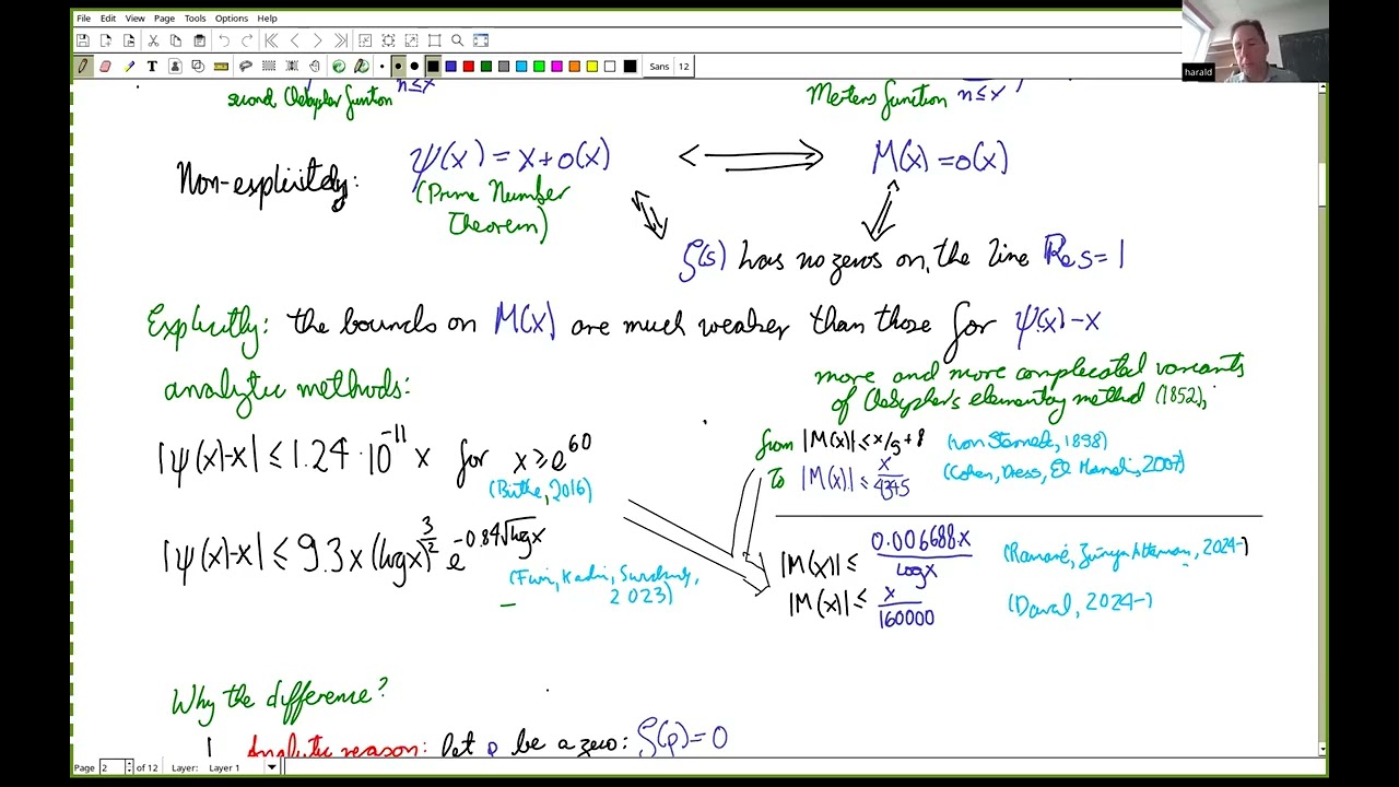
Harald Andrés Helfgott presents new optimal explicit formulas for partial sums of arithmetic functions, specifically focusing on the von Mangoldt function $\Lambda(n)$ and the Möbius function $\mu(n)$. Although these problems are analytically equivalent to statements regarding the zeros of the Riemann zeta function, their quantitative estimates differ significantly due to how analytic methods handle contour shifting. Estimates for sums involving $\Lambda$ benefit from favorable residue properties that allow contours to shift left effectively, whereas explicit bounds for $M(x)$ have historically suffered because standard techniques fail when crossing zero-free regions without yielding constants dependent on unknown distances to near-multiple zeros. Consequently, Helfgott introduces formulas that rely solely on verified data up to a specific height $T$, utilizing error terms proportional to the hyperbolic tangent of $\pi/2T$ for bounded functions like $\mu(n)$, which he proves are sharp by constructing specific oscillating sequences.
To achieve these results, the presentation employs an innovative strategy involving Fourier transforms instead of Mellin transforms to approximate brutal truncations with smoothed sums, thereby avoiding issues related to compact support in holomorphic functions. A key innovation is a "thief-in-the-night" technique where smoothing functions on the real line are replaced by their meromorphic extensions to facilitate necessary contour shifting. The optimization of these smoothing functions draws upon established results from Bohr-Selberg theory regarding best $L^1$ approximations, noting that for non-negative functions like $\Lambda(n)$, optimal performance is achieved by stitching two such approximation functions together. This approach allows the speaker to derive clean human-written proofs within a formal system, resulting in self-contained demonstrations of foundational concepts like the Prime Number Theorem using variants of Vinogradov's method and Diophantine approximation techniques originally explored by Jean-Pierre Kahane.
The computational efficiency of these methods is further enhanced through interpolation formulas optimized with Fast Fourier Transforms (FFT), where zeros are processed via "pinking shears" to create smooth triangular functions rather than being segmented into pieces. This specific processing ensures that coefficients decay quadratically, which guarantees the absolute convergence of the interpolation formula and offers a significant improvement over brute force or standard analytic bounds found in existing literature. By redoing proofs from scratch using combinatorial identities related to Selberg's elementary proof and Kletsky's work, Helfgott establishes explicit error terms like $M(x) = o(x)$ without relying on potentially poor estimates from previous studies. The presentation concludes with a discussion on formalizing these advanced analytic results in Lean using AI tools such as Aristotle, highlighting the necessary updates to libraries like MathLib to incorporate general Riemann-Stieltjes integration required by this rigorous framework.
Read the full video transcript
I'm going to talk about a really basic
problem, that of summing arithmetic
functions. So, of course there's a
formal definition, which is that an
arithmetic function is just a function
on the positive integers to the complex
numbers,
or equivalently a sequence. That's too
general, then we have the definition
that we actually like, namely that it's
a function of that kind that is
interesting to us as number theorists.
Well, that's not really a definition,
that's a social definition.
Something in between the two might be
that an arithmetic function is really a
sequence a n such that the Dirichlet
series A of S
has meromorphic continuation. If not to
the entire plane, then up to a sensible
region. But let's let's say to the to
the entire plane to simplify.
All right. So, two examples of
arithmetic functions, two examples that
we could call paradigmatic without being
too pretentious,
they really serve as examples
of subfamilies are a n
equal to lambda of n, so the von
Mangoldt function, which is basically
the characteristic function of the
primes times log p.
And there the Dirichlet series would
just be minus zeta prime over zeta. And
then you also have um
the Möbius function, which as we know is
just minus one if you have an odd number
of prime divisors and one if you have an
even number of prime divisors. And then
um
A of S is one over zeta of S.
Right. So, the the issue in all of these
is where the poles and what are the
residues.
So, in both cases we know a fair deal
because these functions have poles
precisely where zeta has zeros. And
well, in the first case also where zeta
has a pole at one.
Um
and I have drawn I mean we all hope
I have drawn the zeros of zeta in green
because green is the color of hope. We
hope the Riemann hypothesis is true.
But we have two kinds of partial results
towards the Riemann hypothesis, namely
we can check the Riemann hypothesis
rigorously after
certain
given finite height T.
So that I can draw in blue. The zeros
are really on the line real part equal
to 1/2.
Or we can also show that zero free
region holds. That you know, you have
some sort of narrow ever narrowing
region close to real part equal to one.
And um
I no longer have display problems. Very
good. Um
And there we are guaranteed not to have
zeros. I will really focus here on the
first kind of partial results, namely
let's say that we have verified the
Riemann hypothesis up to height T as we
have. What can we deduce then?
So
I'm having a little computer problem
here.
Yes. Excuse me, one moment.
Yes, hopefully this will work.
Very well. So the idea is always how to
translate information on the poles of
the Dirichlet series to get us estimates
on the partial sums of a n.
Because many of our problems in analytic
number theory reduce
to having estimates on these sums. And
in this talk I will focus on explicit
estimates.
Well, as we will see if you really just
assume
the Riemann hypothesis up to height T,
then that's the sort of estimate you're
interested in.
Um so, on the one hand, you have So, but
let us talk about the non-explicit
regime first, the regime that most of us
are used to working most of the time.
Then, um
psi of x is just the sum of lambda of n
up to x.
And then, the fact that psi of x is x
plus little o of x is just a prime
number theorem.
Then, on the other hand,
so the Mertens function, big M of x, is
the sum of mu of n up to x
for n up to x.
And there, uh you have the statement
that M of x is little o of x.
That's morally morally equivalent to a
prime number theorem. It's also really
equivalent in at least two ways. So,
there is an elementary, though
non-trivial, proof of equivalence
between the two
that is almost as old as the prime
number theorem.
Um and it's also the case, as we know
since uh Vinogradov, that both of these
statements are really equivalent.
Certainly, the fact that this statement
on the left
is equivalent to zeta of s having no
zeros on the line real part equal to
one.
Uh that's Vinogradov. Now, so since the
statement on the zeros of zeta
is equivalent to the prime number
theorem, and it's also equivalent to M
of x being little o of x, the two
statements are equivalent to each other.
Besides the fact that we also already
know that by elementary means.
So, uh the world is beautiful at this
level, and we are used because of this,
we are used to thinking of the problem
of estimating psi of x and the problem
of estimating M of x
as being basically be same.
But here
comes the interesting part that when you
try
sit out of you know, you spend your
entire life your your education consists
in part of being told that they
explicit estimates are not interesting
that you should know that's engineering
or what have you. Well,
substitute your favorite kind of snow
vicious snow viciousness in there that
you really shouldn't look at explicit
estimates. But, say out of curiosity or
because you need explicit estimates, you
look into explicit estimates.
And then you realize that there's
something really interesting going on.
Because the even though these are
supposedly equivalent,
the estimates that we have in the
literature for psi of x
and for m of x are of vastly different
quality.
On the left even even for psi of x the
situation with estimates is more
complicated than what one might naively
expect
from you know, what you know from proofs
of the prime number theorem that you
learn when you first took analytic
number theory.
But, um
nevertheless the situation of of for psi
of x is more or less satisfactory thanks
to dozens of papers.
But, for m of x you also have more than
a dozen papers over time well over
plenty.
But, the situation is very different.
So, on the left what you have is that um
the kind of proof that
we all know and love that this comes
from the level of Busan and and Adamar
can be adapted with a lot of pain thanks
to the work of a lot of people to give
good explicit bounds.
But, those bounds so true in general
pretty much. They start being better
than all other bounds only for x rather
large, when x is bigger than
10 to the 1,600 or so.
Um below that range, you're much better
off
with another kind of bounds, bounds of
the form psi of x minus x is at most
little epsilon times x.
Where little epsilon right now, the
record before our work, was about 10 to
the minus 11. No, and this is true
naturally only for x starting at a
certain point.
But for x up to a certain point, there
are computational bounds, be they brute
force or computational analytic bounds,
which we might talk about at the end.
All right, so the situation is already
more complicated than we thought, but
it's pretty good.
Um it's either the bound is either a
tiny epsilon times x or
um it's this bound that is really little
o of x and of roughly the form that you
would expect, even if 9.3 is a bit
larger than you might have guessed,
uh it's still quite decent.
All right.
But what happens for M of x?
Can you hear me clearly?
What happens for M of x?
Um
well, the first bound on M of x in the
literature,
it's um
that it's at most x over 9 plus 8. That
the proof is in one page. It's by von
Sterneck. It's basically a modification
of uh Chebyshev's uh method from before
the prime number theorem.
That's from the uh 1850s.
Um
however,
uh the problem is that things haven't
really progressed all that much since
then. Or rather, the best bounds that we
have uh are really
more and more baroque versions, and I
say this for
with full respect for lots of good work
and for
Baroque constructions and so forth.
More and more Baroque versions really of
um the von Stern neck Chebyshev method.
These are not analytic bounds. These are
combinatorial methods with coefficients
chosen by trial and error basically.
And where um actually the strongest
bounds which get used all over the place
are in papers that are not really
self-contained and which really
if you read them closely are saying or
not saying things such as if you want
our coefficients, well, we have them in
a floppy disk somewhere.
Um and that's not fantastic from any
point of view. It's not just this this
coefficient 1 over 4,300
is not nearly as good as 10 to the minus
11 and it's not just that these
asymmetries bother some, but also that
um really things become less
self-contained and more complicated.
Though this itself here for But it's
fairly self-contained, but this itself
depends on a long chain of papers.
And then um but what what happened to
this equivalence this supposed
equivalence? Well, if you just try to
use
this equivalence between this statement
and that one, you will get horrible
bounds on m of x. But you can use the
ideas behind this equivalence
to do the following, to combine
these bounds on m of x which are not
analytic, which are combinatorial
with bounds of this form on psi of x
minus x
to get bounds on m of x which are
genuinely of the form little o of x.
They will not be fantastic um but they
will be useful. They will be much weaker
than these ones, but they will be
genuinely useful and I was using those
bounds
uh in uh my work on on on ternary
Goldbach
uh which has been delayed in part
because I you got
uh well, you have seen what I
you are seeing what I saw, namely
I mean you take a trip to the sausage
factory and then you don't want to eat
sausage anymore unless you make it
yourself or what have you.
Or or you decide you will eat something
else instead.
And so you also have bounds a very
recent bound on M of X which is stronger
but it's really based on this result.
It's really a bound of this kind. It's
just that you are really using the fact
that for X below a certain bound you can
use a brute force bound instead. So a
bit more complicated than that but
that's the spirit.
So the real question is why is there
this real at some point even if you
don't care about quantitative estimates
you have to accept that some
quantitative difference are so large
that they become qualitative.
I think it's fair to say that we have a
qualitative difference here.
Just prima facie.
And that's really the case.
Analytic people are not are not being
silly. There was there were really
analytic obstacles.
People were not able to um
get analytic So on the left you have
analytic analytic methods that are more
or less like what you learn in a prime
in a first analytic number theory course
except more complicated because you have
to make things explicit and you have to
be quite clever if you don't want nasty
constants.
But um
on the right the analytic method gets
blocked.
Why?
Why is there this difference?
So there were two good reasons or at
least two reasons that looked good.
Um so two good analytic reasons and as I
will tell you one of them is essential
and the other one is not.
So one of them is the following. It's
not really that Mobius is nasty. It's
it's that lambda is unnaturally nice.
That um
it's uh the Dirichlet series which gets
continued to minus zeta prime over zeta
is naturally nice.
Why?
Well, let rho be a zero.
Then really what we care about when we
work things out, when we shift contours
to the left
is the residue of minus zeta prime over
zeta. But the residue of minus zeta
prime over zeta at zero is something
beautiful.
It's just a multiplicity of the zero.
And we count zeros with multiplicity
anyhow.
So a residue of minus zeta prime over
zeta appearing a so-called explicit
formula is not a problem at all.
You want to
you're already taking that into account
naturally.
So if you count each zero k times where
k is its order, which of course it's
always one, but we don't know that.
Um then
you're basically giving each zero a
weight of one quite naturally.
[clears throat] There's no problem there
whatsoever.
Whereas the residue of
one over zeta is well, goodness knows
what.
Well, it's not really goodness goodness
knows what. It's closely related to the
distance of the nearest zero.
The problem is that we have no control
over that. We believe that zeros cannot
just bunch together as closely as they
want.
But that [clears throat] is felt to be
further off than the Riemann hypothesis.
We don't even know that there are no
double zeros. And just like we don't
know there are no double zeros, we don't
know that there are no zeros which are
almost double, and unspeakably close to
double. These two zeros that are
extremely extraordinarily close to each
other. We don't believe that happens.
But we cannot rule that out.
We can compute zeros up to height T and
show that it doesn't happen there.
But we cannot say that in general it
doesn't
We don't know how to prove that.
Even under our age, we don't know how to
prove that.
So, because of that, we cannot just
shift the contour to the left all the
way to the left
when we are estimating m of x.
We could instead shift the contour
within a zero-free region.
Um and that's what we would do when we
are proving uh non-explicit estimates
when teaching analytic number theory.
But that actually gives pretty ugly
explicit bounds.
Um that's not how you prove, by the way,
explicit bounds for psi of x. You really
do want to shift the contour all the way
to the left.
Um and if you try to do that but for uh
for m of x,
in principle, that's doable, but that
will give you pretty horrible bounds.
Uh and nobody has done that correctly in
the literature. So, there's an incorrect
result on archive.
Um but um somebody should really do that
uh just for comparison, but the result
will be very ugly and fairly useless.
That's the truth.
Um simply because um
our bounds for 1 over zeta within a
zero-free region are so bad. You We get
them by exponentiating really a bound
that is already not fantastic.
Still, somebody should do that and do
that well, but it's it's actually quite
tricky.
I need
All right. So, that's already a serious
difficulty.
Um then there's another thing. I told
you that Well, if we could use We can
check that the residues are We can check
the computer residues
using integral arithmetic. So, up to
high standards, we can really prove that
they are bounded by something uh
for all the zeros of height up to T.
That is of imaginary part up to T.
But then you have another difficulty,
uh which is really more of an
psychological block more than an block,
but it looks like an analytic block.
So, um
how do we bound uh a partial sum? We are
modern people. So, you know, I think
Yeah, everybody who is an organizer is
more or less in my generation, maybe a
bit younger, maybe a bit older. So, we
were told um
to always smooth
uh in part by some people who may be in
the audience. I haven't checked.
Um
So, our advisors told us to always
smooth.
Or
they also told us smoothing is given by
nature.
I'm referring to somebody in particular.
Is he online or not? Which is actually a
deeper statement, but in this case it's
not given by nature. We have to choose a
smoothing.
So, we approximate, being modern people,
um
our sum which has a uh brutal
truncation, as people say in the in in
French, a sharp truncation, by a sum
with a smoothing.
And then you have something nicer and
more civilized than the ones formula.
You have an inverse Mellin transform,
and in here you have the Mellin
transform of your smoothing, your
continuous weight.
Um and then uh if I were, you know, this
would come with a warning, because if
say you were uh I were giving this talk
to young and sensitive um
first year grad students, say,
then somebody might one of them might
stop listening and say, "Aha, I have a
brilliant idea. I'm going to
revolutionize everything. I'm going to
choose an eta such that um
the Mellin transform has compact
support, or at least its restriction to
uh
uh the line
the restriction to the line imaginary
real part equal to one has compact
support. But in my stylus though,
there's an I missing here.
Okay.
Uh why would you want to do that?
Because, um
then, uh we could shift the contour to
real part equal to minus infinity, and
the only residues
uh that we would take be taking into
into account would be uh the residues
with imaginary part at most T, and we
would be done.
Now, of course, the problem is that's
completely impossible. You cannot have a
million trans- The million transform is
holomorphic within a band.
Um uh within a band. And the holomorphic
function just can- cannot have compact
support. Its restriction to a line
cannot have compact support. Even even
the continuous even if the uh you are
holomorphic within a band uh we within a
band, and you continue your function
continuously, your holomorphic function
just continuously to the
to the border of the band, uh the
function cannot be compactly supported
there on the border. So, it's a little
bit subtler.
Uh and so, you know, the graduate
student just the imaginary first-year
graduate student goes home and cries.
Dreams are dashed. You fall off a purple
cloud.
Um yeah.
Okay.
Uh
sad story.
Uh imaginary story.
Um however, I claim that you can you can
do something that is as good as that.
We can manage to use only the residues
of, say, one over zeta with imaginary
part with absolute value at most T, and
we can do that optimally.
And the zeros of zeta with imaginary
part greater than T simply do not appear
at all.
And so, we have two main theorems here.
Um if you find that it is a bit full,
you can
decide to use to look only at half of
the screen, you are free to do that.
Yes, Henrik, I meant you.
And I I I I did mean that you So, I
should credit the Sattler version of the
two statements to Henrik.
Okay?
Namely, that smoothing is given by
nation.
>> Yes.
>> Sorry?
>> I expected you meant me.
>> Yes. Yes. Not The second one was you. Uh
yeah.
>> At any rate, moves moves every time.
>> Excellent.
>> Okay.
Bye.
>> Of course, as we will see, one should
not be too picky. Often,
um
you don't want a smooth smoothing as in
C infinity.
Sometimes, C1 is optimal, in fact, or
even less than C1. We We shall see.
>> And be more right.
>> Excellent.
Very good.
So, if this is too confusing, just look
at your favorite half of the screen. So,
if you care about bounded functions,
such as mu of n, look at the left half
of the screen.
If you care about non-negative
functions, such as lambda of n, look at
the right half of the screen.
Why do you have to assume one or the
other? Well, you don't really have to,
but having one one assumption or the
other really simplifies things vastly,
and having one of these two assumptions
allows us to give a fully general
statement. So, mu of n and lambda of n
become really special cases.
So, let I because the formula is a bit
nicer for mu of n, let me focus on mu of
n.
So, for mu of n,
as for
for mu of n, you generally get
a
an explicit formula
that involves only uh, the zeros with
imaginary part up to T.
Because here, so this is the formula.
So, what does this mean?
So, uh, for me epsilon means something
extremely In fact, epsilon is tiny both
in theory and practice. Epsilon is
little o of one, and it's also really,
really tiny. Uh, so it it's less than
one over T squared. So, for where T you
should think of the height up to which
you verify things, you should think of
it as being at least 10 to the 9 even on
your desktop. In fact, you ask a a very
good programmer, in this case David
Platt, and he will carry out the
computation much higher than that.
Um,
so epsilon is really tiny. For me, iota
is something bigger than epsilon, but
still quite small.
That's the way in which normal people
use iota. Um, and what is iota here?
Iota is some quantity
smaller than uh, hyperbolic tangent of
pi over 2T, which is of course almost pi
over 2T.
Um, this we will see, this is really
interesting This is really there. This
is optimal in in two strong senses, we
shall see.
So, you have you cannot avoid having
this little term that is smaller than pi
over 2T. And more precisely, it's
bounded by hyperbolic tangent of pi over
2T.
And there here you have what you expect
in an explicit formula. It's a sum over
zeros, but you what you don't over
poles, but what you don't expect it say
that it's a sum only over those poles
that have imaginary part at most T.
And then what you do expect or almost is
what you have here, so a residue.
The residue at rho of I of S times X to
the S minus 1 times a weight. And the
weight is the optimal weight, which
turns out to be beautiful as optimal
things sometimes are. At least I can it
beautiful because it's basically just
hyperbolic cotangent minus minus a
constant which is hyperbolic tangent of
pi over 2t.
So, the weight is just hyperbolic
cotangent which is because s is
something vertical, it's it's really
basically cotangent.
Right.
And and that's really it.
There's not much and much else to it.
The formula for a n non-negative is a
bit more complicated and you do have
some
other o star terms
uh which don't dominate but you still
have to take care of things. It's a bit
more painful and we will later see why.
O star just means something with
implicit constant at most one.
But again, you have um
that yeah, you have uh trigonometric
functions lurking in.
All right. Before we see where all of
these functions come from, let us see
what they give us. And you might think
that these results are ugly because, you
know, though they are one line in this
case, this one is one line, you need to
explain what the terms are. Well, let's
let's see.
So, first let let me just I've written
it down to to explain that I'm not
lying. That here
the iotas here
all of these terms
pi over t cotan No, actually this term
this term plays a role of one. This is
very funny.
That you will see this phenomenon later
but the iota here that the role of iota
here is played by pi over t.
And whereas here is tan hyperbolic
tangent of pi over t.
And these these intrinsic tiny but
constant error terms are really optimal.
In what sense? That we can actually
construct Dirichlet series that don't
have poles
you we can construct sequences such that
the Dirichlet series don't have poles
with imaginary part bounded by t at all.
They have no poles there.
No poles whatsoever. The sum over poles
is empty,
but they still oscillate.
They oscillate
and by how much?
Exactly by in this case for A and
bounded by hyperbolic tangent of pi over
2t. Or it would be pi over t in the case
of non-negative functions.
So we can actually have construct
bounded A and
such that
the the sums don't obey the prime number
theorem. They miss it just by this tiny
term hyperbolic tangent. They oscillate
by that.
Now, I'm claiming that these results are
optimal. I'm also claiming that they're
optimal in general. And I but for mu one
can do better. So what how can you do
better than optimal result? Well, mu has
um
uh well, it's not just that it's optimal
given a verification up to T. I claim
that you you can do better just with
some
verification of zeros up to T.
Simply because mu of n is not has
support on the square-free integers. So
you should be able to win that to gain
that factor of 6 over pi squared and and
we are able to.
So in the end um
we have pretty clean bounds.
So we get for M of X
um using a rigorous computation of the
residues of one over zeta
for imaginary part of the 10 to the 10,
we get that M of X is bounded by 3 over
pi times X over 10 to the 10
plus something in this case a constant
times square root of X. You know, in
general, you know,
we
this is not guaranteed to be a constant.
It's a sum over zeros, but it turns out
to grow very reasonably. There's some
cancellation here. No, actually this is
without cancellation. We will later talk
about cancellation, but without even
without cancellation, this is something
reasonable. So you get this bound which
you should compare to what we had
before.
Awesome.
This anonymous bound, valid for all x
greater than equal to one.
And this is the
10 to the 10 is really the level up to
which we have checked t and 3 over pi is
precisely zeta of 2 * pi over 2.
Now, in fact,
we also improve on existing bounds for
lambda of n. I mean, we improve them by
less because the results that existed
were better.
And in fact, in some sense, the the
optimal bounds that we get for
non-negative functions are worse by a
factor of two.
In this case, they are they are better
simply because the Riemann hypothesis
has already been checked
up to height 3 * 10 to the 12 by Platt
and Trudgian.
And you don't need to compute residues
here.
But you get something very funny that I
did not expect. Maybe some people
in the audience knew this, but I never
knew that I was we were going to get
an error interval for psi of x that is
not centered on x. It's a little bit
off-centered. Of course, the error
interval contains x, otherwise you know,
the world would collapse.
But still, it's something very funny
that I did not expect.
And then you have this iota, which just
to simplify the iota plus the epsilon is
bounded by pi over t minus one times x.
So, we can give this general result that
if RH holds
for all imaginary for all zeros which
imaginary part up to t,
this should be an absolute value,
obviously.
Then,
you have this formula.
And this is
optimal, as I said, in this generality,
you know, when you want a result valid
for non-negative functions.
You are not using a zero-free region at
all here.
This coefficient for square root of x is
basically what you could expect, except
that we actually get for free
a little bit a small gain on what people
had before, which was these, just
because
the weight function decreases, no?
So, unconditionally we get the
following, that for all x greater than
or equal to 1 this holds. Now, this
constant is a little bit uglier for
it's an interesting phenomenon, but this
works quite nicely.
All right. Now that we are happy that we
have results, we have, I guess, 20
minutes for the proof? 25 minutes for
the proof?
Very good.
So, what is the proof strategy?
So, again, smooth smooth smooth or
We will approximate one not by an
arbitrary eta and then work with Mellin
transform of eta. We already know know
that that could lead us into trouble.
We will approximate it by a Fourier
transform, phi hat. Okay?
And then we don't use the inverse Mellin
transform. We just use
Basically, we don't even have to hurt
the
the Fourier inversions here. We just use
the definition of the Fourier transform
and we get this, which is roughly
analogous to the Mellin inversion
formula, but in fact it you can prove it
in a paragraph.
And this is not new. Statements like
this exist um
uh
in some form, not sometimes we say hard
switched, but this statement
exists in proof of the Wiener-Ikehara
theorem. Um
and uh you even have there in in proofs
via Wiener-Ikehara of the prime number
theorem the idea that you can choose phi
to So, here here you don't you're not
phi just needs to be defined on the real
line. So, you are you don't have to
assume
you you are not hurting holomorphic
functions at all. And phi particular
does not have phi I be of compact
support. That's completely fair.
Uh phi yes has to be in L1. Its Fourier
transform should be in L1, but that's
completely compatible with being of
compact support. You can have for
instance trian- the triangle, or you
could have the truncated cosine. You can
have whatever you want.
It's It's a very you know soft condition
that phi be in L1, phi hat be in L1, and
you let's say that you also impose a
condition that phi be of compact
support. Support in minus one comma one,
and then this um improper integral
becomes proper. It just becomes an
integral from one minus IT to one plus
IT. Again, nothing new here because the
proof of inner product had a status this
way.
Now, the following step is already new.
So, um surprisingly so
uh
we want to know since we we're going to
do this, okay? But we we said that we
are going to approximate our brutal
truncation by uh uh trun- by a sum that
is weighted by phi hat. So, what is the
difference between the sum that we want
and the sum we actually estimate?
So, um you know, this is the sum we will
actually estimate,
and the sum we want is the sum with a
brutal truncation. So, we want to
because AN is bounded, we are doing that
version of the proof, we want to bound
this quantity here.
Now, just by some change of variables um
we end up having this sum over here.
That's nothing.
And then the following step is
surprisingly already new. So, this looks
like an L1 bound,
and it is generally
basically an L1 bound. You can You can
bound this sum here
by 2 pi over T times the difference in
L1 norm between phi hat and I over in
the real line plus some tiny tiny tiny
error terms, which um depend on being
given that you know, you're given the
input that phi hat minus i t case
quadratically. Where in fact I you
barely need it here. I here um here and
here I is not um
uh the characteristic function of an
interval. Here by I I mean a truncated
exponential.
Okay.
So uh
everything this is bounded by 2 pi over
t times the difference in L1 norm, the
distance in L1 norm between phi hat and
the truncated exponential and you have
some very terms coming from some tail
bounds on phi hat basically.
Uh here, you know, the this is
important. If you just try to use
the the tail bounds and work only with
that, you're going to get something very
suboptimal. You should really see this
as an L1 bound. Aided a bit by a by a
tail bound.
Okay.
Now comes an interesting step.
Uh how many of you have played Mafia or
Werewolf?
Okay. So um
we uh have this integral here, this
integral over the finite segment 1 minus
i t 1 plus i t.
Now everybody goes to sleep.
Now, close your eyes. A benevolent
thief, a philanthropic thief, comes in
the night
and replaces little phi, which is just
defined on the real line, by big phi.
Big phi is meromorphic. And not only is
it meromorphic,
but uh it's identical to phi not not on
the whole real line. That would be
impossible. Just on the segment minus 1
{comma} 1. That's
the case.
Now everybody wake up.
So the value of our integral has not
changed
because we have just replaced little
phi, the thief replaced little phi by
big phi,
uh Uh, and you know, and the argument
goes from minus one to one, so there's
no difference here.
You still have this ugly image over T,
but you're on a line, so this is just S
minus one over IT. So, you now have a
beautiful very a beautiful complex
integral.
And now, you can shift the contour over
to the left. You you get these skid
marks, horizontal skid marks, but they
are no big deal. Certainly for mu of n,
they contribute something very very
tiny.
Uh, that's these contour integrals, so
you're horizontal contour integrals, and
then you just are capturing the residues
given by the zeros of height up to T.
So, by the way, the closest anybody has
got to these, and this was the main
inspiration, you will find these in
Ramana not these, but you will find
something a bit like these in Ramana
Ramare
because um at when they So, Ramare
really made me aware or made many people
aware a long time ago how frustrating
this lack of parallel between mu of x
and psi of x was.
But, interestingly, I think the closest
that uh
that he came to these was in a paper on
a different problem, a paper by
Ramanujan and Ramare. And Ramana had
also worked
on um
variations of Ingham-Jessen
where they were using they were not
looking at this problem in full
generality, and they did not have the
previous bound on the one norms, but
they were working with piecewise
polynomial functions.
Uh,
a piecewise polynomial phi indeed. And
and of course the issue with a piecewise
polynomial phi
is well, a polynomial isn't entire. So,
then you can shift.
Yeah. So, that's the
the
I think that it's important to give them
credit for that.
But, you really should look at this
problem in full generality. And in full
generality, what we you want is a thief
in the night. Whenever you you have
little phi such that you have a thief in
the night, you can in fact shift the
contour.
Yeah, somebody say something.
No, not yet.
Um
All right.
So,
uh
Very good. Very good. There's a finite
number of these poles, and you can just
compute the residues or really ask David
Glad to compute them.
Um
and uh this fantastic. Of course, I was
telling you that I was giving you the
version for not the bounded version.
What about the non-negative version? For
the non-negative version, you don't even
need this.
Uh number two. However, for the
non-negative version, um
you you will see that we get a bit lucky
with phi that you will find that our for
our optimal phi, there really is a big
phi.
Uh for the optimal phi for A and
non-negative, uh you have to paste two
phis, two big phis. So, um uh and you
have to not be you should think of them
as them as being sewed together, and you
you Now, you have a little suture here,
and that gets a little bit messy, but
it's not too bad. These are the suture
lines, so to speak.
Okay.
Let's proceed. So, the problem is to
find phi such that phi hat minus I, I
being a truncated exponential, is
minimal in L1 in L1 norm.
But, that's uh
an optimization problem of known type.
And in fact, it it's has been solved uh
over the course of time for by different
sets of people for different
uh
uh different things. Uh certainly for
the for the functions we we are
considering here, bounded functions,
non-negative functions,
it has been solved. So, in the special
case that would come if we were
estimating as we can sums of the form
lambda n over n, that was solved by Bohr
and Selberg. They never published or
Bohr never published, and his student
Riedel date, and he didn't actually
publish in the paper. Well, never mind.
Uh they had their own publication. It's
difficult to give a precise date, but
this is known to people since the '70s.
Uh and then there's um but we really
need a more general thing. So,
Beurling-Selberg has been used a lot in
analytic number theory, so it's a bit
surprising that this hasn't been done.
But we really need a more general thing,
but these things that are known to
number theorists as well. So, Graham and
Vaaler
that's uh they solved the problem, the
right problem for uh sums of lambda of
n. And for uh sums of mu of n, really
the the solution is due to Vaaler and to
Carneiro-Litman.
Because what are the problems here? It
depends on the constraints. So, um if
you have bounded functions, it's really
just that.
You want the phi which supports on minus
one comma one such that uh the
difference between phi hat and I is
minimal in L1 norm.
Uh
no other constraints. Yes, that the
support of phi
is um is in minus one comma one, so it's
it's it's continuous at minus one,
right? It's continuous everywhere,
that's all.
And then then it's Yeah, it's known what
what uh what the problem is.
So, um it's this [snorts] thing on the
left.
So, um it is approximate what people
call approximate. So, this is what you
get from mu of n over n. This is closest
to Beurling-Selberg.
Uh that was uh Graham uh no, Vaaler.
That was Vaaler.
No, that was Graham-Vaaler. And then
Vaaler
um no, Vaaler was this, Graham-Vaaler
was this. Uh no, I'm getting this
completely backwards. So, this was
Vaaler and this was Carneiro-Litman.
Right.
So, these are the best approximates. We
can plot them quite nicely.
Uh I mean, they are special functions,
but it has um the approximates, but we
will see that they are Fourier
transforms of very nice things, not
really special functions.
And um whereas uh when you also have the
added condition which you need for when
the functions are not bounded but
non-negative that the function your
approximate might
are majorants or minorants of the
functions you're approximating. There
you have the in fact more familiar
Bolling Selberg problem. People have
seen this plot before probably. And here
is if you have the truncated
exponential.
Notice how these functions
are equal to the function they're
approximating at the
integers except for zero in this case.
And at all half integers in this case.
That's not a coincidence.
There are several ways to do this. You
can see this by calculus of variations.
I don't see it standard way in the
literature. It seems as an interesting
heuristic.
That's how we first saw it before we
realized that it was not just inspired
by the literature but contained in the
literature. Or you can do it in other
ways. But this is really not not chance.
You end up using an interpolation
formula.
And something that is really not clear
is stated in the literature because
people tend to phrase people tend to
work most of these papers work out phi
hat not phi itself. Most of them is that
phi is actually much nicer than phi hat.
Phi hat is already nice enough. It's a
sum. You can write it in terms of the
digamma function sometimes or the large
function. But phi is something
beautiful. Phi is something you can
write in terms of hyper- hyperbolic
trigonometric functions.
Well, really just trigonometric plane or
trigonometric functions because you get
that
as um
Yeah, you
you you get that by you know you get a Q
series from interpolation formula and
every and precisely because it is a
trigon- a trigonometric function but
basically a trigon- a trigonometric
function shifted a bit in the complex
plane.
Um yeah, you get that because
trigonometric functions are meromorphic.
So, phi the optimal phi is a
trigonometric function restricted to
minus one comma one, so big phi always
exists. Or for majorants and minorants,
you really get something of this kind,
you know, a phi little circle plus sine
of t and as I said, you have two
functions summed together close to the
x-axis.
And this is the greatest contribution of
AI to this paper, namely it
um I mean
So I I I have to credit, I think ChatGPT
with This is just a center. Uh so this
is a proof that this half Fourier, this
is supposed to be Fourier and half
analytic. So you are really um
if any you remember anything from uh the
proof, it should be this.
Right? So you start as in a free
analytic proof of the prime number
theorem, and then you shift gears
entirely and it becomes a complex
analytic proof.
Okay, what now?
So
uh yeah, so this is optimal. You should
So you can and you should redo large
parts of explicit analytic number theory
now. This sounds insufferable, but it's
true
because much reduces to bounds on psi of
x and mu of x, and the same techniques
apply to many other L-functions. Uh it's
you know, I don't I
you have to I have to be a bit careful,
but I would say morally speaking that
this applies to a class of functions
broader than Selberg class because you
don't really need a functional equation,
even though it's helpful if you really
want to shift to minus infinity.
And there's really no point in waiting
since bounds are essentially optimal as
a function of t. Certainly the leading
terms are.
Um
and in fact, there's now a team of
people um
of people and not people who are uh and
AI really does come into play there for
working at formalizing this in Lean.
Uh there is an entire project to to do I
mean, it's really important to, you
know, clean up the social factory. And
this has become part of this. So, uh
formalizing this paper these two papers
has become a priority. I think both
should be a priority, but people have
started with fire effects.
Uh I've had a small role in that
formalization effort.
Um
I'm not really fluent in Lean by any
stretch of the imagination, but there
were all sorts of surprises as to what
and how they had not been formalized.
Um okay, people people have told me not
MathLib, people have told me not to say
this, but I will say this. As far as
number theories are concerned,
MathLib has all sorts of sophisticated
and beautiful things, but it did not
have integration by parts in the
generality that we wanted because it had
integration by parts when for two
functions that are in C1, but of course
that's not enough. We want integration
by parts when one function is C1 and the
other function is of bounded
And that was not in MathLib and could
not be in MathLib because um the theory
of uh
Lebesgue-Stieltjes integration was not
ready yet and it will not be ready yet
for a couple of years, I think.
Um and uh people in MathLib thought that
Riemann integration was beneath them, I
think. They had something more general
called box integral, which is helpful,
but it was not, you know, it only the
basic theory was worked out. So,
Riemann-Stieltjes integration was not
there.
So, something that I did, everybody
wants to hear about AI nowadays.
So, uh something I did in January was I
was playing with AI. Uh and AI can
already form help in formalizing things
badly. It produces ugly code often, but
it's very good as a um proof of concept.
So, I found that um there there is uh
Aristotle. It's uh
yes, it's it's an AI tool, but my my
much of the time you can also just use
by now really powerful general LLMs
uh that um if you choose your textbook
well, it can sometimes chew on a
textbook for a couple of the few pages
of a textbook and spit out
formalized uh code. And so for instance,
I found that um
textbooks that I like were also liked by
Aristotle the AI. So
uh I I think um
uh Zigmond is fantastic and Aristotle
felt the same way. Uh and um of course
the code that uh
Aristotle produced was much uglier than
Zigmond,
but this uh but I
by mid-February I had that you could use
Zigmond and also appendix A in um
Montgomery Vol. 1 to get uh
to formalize
enough Riemann-Stieltjes integration for
the purposes of analytic number theory
for many purposes.
In what we really care is that we are
able to work um
to have uh
that F hat decays quadratically when F
is of bounded variation, right? And that
comes from integration by parts of the
generality that we need and that was not
there in MathLib. Or also we need there
was a statement in in MathLib. MathLib
people, please take this as friendly
criticism that said literally, "This is
the most general statement of the
Poisson summation formula." And it was
not a statement of the generality we
need in analytic number theory because
it assumed uh you know uh that F was
nicer than many It was It was assuming
that F was C1. And we want to we don't
we we we often want Poisson sum in the
Poisson summation formula
for functions that are not necessarily
C1.
Okay.
So what what has really happened there
is that people were
delighted and grossed out by how ugly
the Lean code was.
And uh people got together including me,
but I you know, as he said, I'm I'm bad
at lean still, uh in May and a team of
people at I sum, I should really have
written down all their names, but you
can look them up in I sum and I think
this will be uploaded and you will see
everybody including young people that
should be given lots of credit. In a
week people managed to redo at least a
basic Riemann-Stieltjes integration in
appendix A of
Montgomery von, and now it's really
really clean and done by humans,
uh and people will be able to use that
and build on that to to be able to
to have what we need in analytic number
theory.
In particular, now we have integration
by parts finally in the generality we
need. Somebody's in the chat.
Uh yes, Henrik, later. One moment.
Do you have a mythological animal that
is Ah, yes.
Yeah, but it's the wrong half of the
elephant.
Well, I do not know. We we shall talk
about that later.
At any rate,
um
yeah.
Okay.
Moreover, there are some other things in
the next 4 minutes that you get many
other things. Let's backtrack from
formalization, let's backtrack from AI
and so forth. Let's get back to human
classical things. So, first of all, just
we weren't intending to but we get a
self-contained proof, yet another
self-contained proof of PNT early on for
free. As in, you know, in in section two
we're just building up foundations and
then
in section 3.1 of both papers we work
out a self-contained proof of PNT
because in section 3.1 we get
Yeah, I should really say that what we
get is that um
the statement that is equivalent to PNT
elementarily because we get very very
easily.
So, it's it's really a variant of
Vinogradov but it's really very clean
and and short.
I've been frustrated trying to give
frustrated trying to give Vinogradov
in class.
And so, you get
that a very, very clean Vinogradov
Vinogradov type proof just in a
paragraph
of the statement that m of x is little o
of x just given the basic theory that we
had to develop anyhow. in particular
Not not not three or four, just just
these bounds. So, just using one and
two, which we need anyhow, we get
basically for free Vinogradov for m of x
equal to little o of x.
Now, of course, I said self-contained
and you could say, "Vinogradov, you are
not self-contained. You still have to
use the
the ancient trigonometric trick or
something which Cauchy-Schwarz to get
that you have no zeros
with
real part of one." But then, when I was
giving this talk on an earlier version
of this talk in Nancy, and then our tone
pointed out, "Harald, you may want to
look at something that Jean-Pierre
Kahane did
a proof of the prime number theorem."
And indeed, you can give
what is basically a variant of the first
half of Kahane's proof
to show in a way that uses again the
foundation section of the psi of x the
non-negative paper that zeta of 1 + it
does not vanish.
Yeah, but zeta does not vanish in the
real part of one.
Now, I I I like to make it to do it
differently. Again, it's two paragraphs.
Yes, use a bit of Diophantine
approximation. Maybe
it would be it's maybe Kahane would feel
that it's a bit impure. He's not now.
He's unfortunately no longer with us.
But it's turns out quite nicely.
Okay, but that's cute and all. Now,
let's uh
go for things that we intend to do, but
people are welcome to try their hand at
it because we are already sketching them
in final remarks. They will be a pain to
do, but um
so, what about bounds of the form
m of x is little o of x, but explicit
bounds? As I said,
all such bounds in literature are based
on bounds of the form m of x
uh bounded by epsilon x. So, we could
redo the old papers to get bounds of the
form m of x
little o of x, but in
but explicit bounds. But, in fact, it's
much better to use the idea there and
redo everything, do everything from
scratch. Because the basic idea is to
use a combinat- combinatorial identity.
Uh and by the way, something that
came
So, did somebody Yeah, I think this also
came out came from
uh
I think Balazard pointed out to me that
I might in these combinatorial
identities,
No, it is some book in a book by
Balazard. There's these combinatorial
identities that people use that are
related to Scherk-Selberg. I mean, all
communi- lots of combinatorial
identities in number theory are related
to each other.
Um one of them is very funny. Um
You you could see this as being related
to elementary proofs of the prime number
theorem. Uh in fact, in particular, I
say that think this is closest. This was
pointed out by Balazard
to um
the the combinatorial identities that
people use to prove m of x is little o
of x.
This is closest to um Kaletsky's variant
of the version of two Soviet
mathematicians, I've forgotten, sorry,
of uh Selberg's uh Selberg or
Selberg-Erdos, but let's say Selberg's
proof, elementary proof. Um
and by Kaletsky, I do mean the
economist. That's a long story.
Um
uh and here um
Yeah, but so, that's the idea that
existed, but you really want to use
those identities and do everything from
scratch. Why? Because
I wrote these
explicit formulas not just out of say
this and I mean the bounds may look
clean and all, but it's better to have
an explicit formula because you can plug
in an explicit formula into something
else and you can
play with it. You can do all sorts of
things with this explicit formula.
Um and you can get cancellation. Even
if, you know, you don't assume anything
about the residues, you can get
cancellation. And that's precisely what
happens. And you know, this is only
sketched in the in the paper at the end,
but you really do get even better
balance than what we would get.
Because just by by using these bounds,
not just using these bounds, should
correct myself, but really using the
explicit formula.
And the other thing is that I talked
briefly about analytic computational
bounds in that it's not just that you
have brute force bounds, then epsilon X
bounds and then little o of X bounds.
There's this twilight zone here between
brute force bounds and analytic bounds
of the type epsilon X, analytic
computational bounds. So there's a paper
there due to Buthe and basic idea is
implicit in Odlyzko.
Um but Buthe is really using a function
that was optimized that is in Odlyzko
and um
somebody else, but
uh that is really optimized for a
different purpose and you should not use
that.
Um
you should use other functions
uh
but moreover, uh what you but the basic
idea is good. The basic idea is that you
want to use interpolation formulas and
the fast Fourier transform.
But you cannot do the fast Fourier
transform on 10 to the 12 zeros and 10
to the 10 zeros. You chop things into
pieces, but here comes the how you can
improve things vastly, we believe. We
shall see how big the improvement is at
the end.
You shouldn't chop things brutally.
Always smooth, remember.
Um you should or always move in a
continuous way at least.
Instead of chopping chopping the zeros,
think of it as being the the line real
part equal to 1/2. Instead of chopping
the this this line parallel to the Y
axis brutally into segments, you should
chop them with um shearing shearing
pinks. No, pinking shears, pinking
shears, right? Uh those crocodile type
scissors. So, you get some these nice
beautiful triangular functions. Two of
them added together give you a constant
function.
And then what happens is Fejer happens
that you end up having an interpolation
formula
where the coefficients decay
quadratically. So, your interpolation
formula converges absolutely. So,
everything works out much more nicely
computationally and otherwise.
And I think this is new. If this is not
new, people should tell me. And they
should have other applications as well.
Okay.
My time is up. I have um another slide
that is not part of the talk, but just
as an answer to a certain kind of
question. Very good. Thank you.