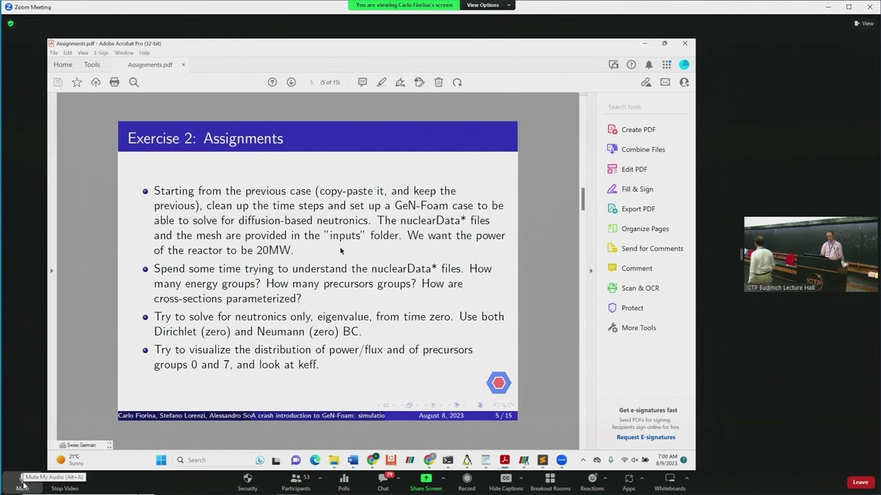
Group Activity 1, Multiphysics simulation of the MSFR using OpenFOAM - PM

um can you hear me now online yes no yes yes I guess we were just looking at uh the results from assignments one and I just said about assignment two uh that I will give you additional time to work on it and if you have questions feel free to ask and I have been asked here to if we can plot velocity as arrows instead of colors the answer is yes and usually you use a glyph she's up there in part of you what was that um you apply after a long time usually you see things oh that was ugly well you have to work on it I will find the solution to this keep doing the exercise too um I guess your hour because you have to decide which parameters so you have to decide which Vector to use and we want to use U the velocity after a while give me a sec ular race doing it like that oh yeah now you can it's uh you have to select glyph and then you have to set that orientation arrays based on velocity and the scale array is based on velocity now you have a lot of arrows you can reduce them now we have 5 000 points I think you can do one thousand and you can remove these and only see the arrows then you can play around with the size of the Arrows with the color of the arrows you can do many things but this is not really open form related this is part of you related it's just and not typical in part of you you can find quite a bit of documentation online now to use paraview and it's the same if you're using value for open form or for any other tool you're welcome foreign for those that are online I've been asked why there are two default fluxes the reason is that when you need to do sp3 instead of diffusion you need to provide initial and Boundary condition for the flux and for the first moment of the fly for the second moment of the flux so in our case you're doing diffusion you can forget about the second default flux foreign what's the key effect you obtained group is there anyone from group one was Decay effective huh sure group two anyone 1.4 Raise Your Voice 1.4 oh six this is okay effective don't be shy with number 1.406 give me another two six another one let's get to PCM at least five okay and this is for a zero gradient or for a fixed value because you should have a fixed value and a zero gradient boundary condition to zero gradient and do you also have results for the fixed value okay that's the same thing for everyone group one second fix fixed value how much is the same okay three zero point five that is the problem zero point 0.439 give me another number zero seven uh group four interesting you're gonna be interesting to figure out what changed because now the funny thing is that yesterday I obtained both and I don't know why but we'll try to figure out why so in the morning yesterday or team one and afternoon the other I think it's a matter of which temperature we are solving it at but let's see let's try to do it together so um I'll tell you what I would do hopefully I will remember to do all of it would be nice so um let me get the folders so if you'd get a wrong number don't be worried sometimes it can be that you forget to set a little parameter and no transform is Big sometimes you need time to go through all of it and make sure that everything is correct I said even myself yesterday did it and opened two different care effective and I think it was because at some point I forgot to set a temperature somewhere anyway so what I would do is um well I what I already did while waiting I copy pasted the case into a starting case too just not to lose what I did before um so this is what we had from exercise one and as I said we have a lot of inputs that are given in the input folder and I said that there are nuclear data and there is a mesh and you need both and you need both where well in the neutron in the neutral region so you're going to constant you're into neutral region you have a poly mesh you want to change it into the new polymesh can you leave it like this no you need to change the name it has to be called a polymesh so we call it polymesh then we have all the nuclear data that were in there that we don't like because they were kind of dummy files with no content or very little content and we want those that I gave you that includes real cross-section data put it in there as I said the idea is let's take a look it's gonna be small but I will do it anyway because you can open it on your computer you look into it you will see things like Energy Group 6 precursor groups eight so we are solving for six energy groups eight precursor groups and we have different cross sections for the heat exchanger intermediate circuit main Etc and you will see that cross-sections are each one of them is into six groups yes it is there for a later exercise it's not no not at all now I mean in open form you can throw in random files it's we simply not read them and I ask you to check parameterization and nuclear data axial expansion you look at it and there's nothing well of course because we don't have a cross-sections for axial expansion this is for fast reactor for solid fuel fast reactor there's nothing in there so we don't parameterize for that uh what about the cool nothing because our coolant is the fuel what about fuel temperature there you have something if you look at it you will see that the cross sections are slightly different than those in nuclear data these are cross-sections that are valid for a different temperature this is how we parameterize the cross section which give longer sections set at the nominal temperature macro section Step at the perturb temperature and we do an interpolation so we are parameterizing our cross-section based on the temperature of our fuel coolant we call it fuel here because it's a molten salt reactor so what's in there that we may need to change so we have our nuclear data we have them parameterized we have controvert movement I haven't mentioned Contour roads so we don't touch it we have the mesh What About neutronic Properties and it's a bit small but it's already diffusion we are happy we keep it we want it to have a diffusion but it says eigenvalue false we want it true it was in the assignment we want an eigenvalue solution so we set eigenvalue neutronics to true so now we look into this and we realize we have touched everything we wanted to touch so we forget about constant hopefully I did everything um we don't touch fluid we don't touch thermomechanic because we are doing just neutronics and then we look into system and of course we would like to touch the control dict um we do it now uh it's small so let me do it because this is important I want to do it in a way that you see what we do so we go to our starting case two and we look at system contradict and you look at it as usual you have a start time okay we start from zero you have an end time and we don't care about the time as I said before these are all time steps we want to Simply iterate and I said we would like to have approximately 100 iterations so if our start time is zero and our end time is 10 what's the delta T to get to 100 iterations 0.1 right 0.1 time steps we do it 100 times we will get to 10 seconds because this is the way we iterate 100 times in open form some things you don't really care about standard open from things what do we want to solve for I said we want to solve only for neutronics so no fluid mechanics no energy solutronics true salt term mechanics false liquid fuel stays as it was just true and just time step do we need it no we are not doing Thermo Hydraulics we don't want to adjust we just want to run 100 iterations so we want our time step to stay 0.1 and get to 10 in 100 iterations this is how we set iterations we use a fake time stepping what happens if you leave adjust time step to false well it will try to adjust your time step based on current number and it is not calculating the current number so you may run into some problem um the rest we don't care we have questions about this contradict does these times the fake time stepping make sense to you not really maybe a little bit you won't write it 100 times we do 100 time step of 0.1 that will not enter anyway but just force open foam to do 100 Solutions we will be in a loop if we start okay I solve one am I at the end now I need to solve once again once again once again for 100 times that's how we create iteration and since we are solving for eigenvalue the D DT the derivative over time has been taken off so we don't really care if our time step is 0.1110 as far as we do it 100 times It's Tricky this is a very open foamish way of doing things because open phone was born for cfd and you always have time somehow so we do it this way what else am I missing or I said that we need to set the power to 20 megawatts and I said that this thing is inside the reactor state how do I find reactor State you can locate you can grab you can think where it could be you can imagine that reactive state may change over time right so the most logical place for it to be is in the time folders so you get to not here you get into your time folder from zero could be in neutral region is not and I'm sorry about that this is again a way we have an open form because in these folders we typically have fields a reactor state has a key effective and power it's not a field we keep those things in something called uniform and in there there is something called reactor state if you cannot find the tube the rapidly located or best thing when you are alone at home and you want to do this thing before doing anything you look everything that there is inside your folder you want to familiarize with every file that is in there and while doing that you will bump into something called reactor state that has a power and a k effect we said that our Target power is 20 or you look at the documentation if you have you know two three hours with the documentation these things are explained um so we have our 20 megawatts to the seven right we said we want two megawatts so well not of zeros for not much two to the seven Watts this is 20 megawatts what about K effective well okay effective is what we want to find does it make sense to give a k effective in there at the beginning kinda this is the initial condition it is you know when you set a new field you set an initial condition you also should do it for K effective it's the initial guess that you provide if not change much but this is going to make your computation faster so another thing that we need initial and boundary conditions many of you noticed that there are default flags and the default flux too full flux 2 this is for sp3 simulations you don't need it uh default flux let me open it from the terminal system zero now what you had here was clearly wrong we were giving a fixed value to everything and uh well it's not completely wrong there are at least two things that were wrong which is the boundary conditions for the wedges so we are doing 2D and you need your front and back to be treated as wedges I don't remember the name of the front and back front and back okay so what you need to do was to create two things that are called well I can actually do it the right way front front type Edge oh yeah sorry right double check why I think it's the first one it finds more relatively short it's the opposite you sure okay I will try here the question is you may wonder why we are discussing is because this thing it says all Fields equal to fixed value and we are wondering if we don't remember if open form gets the first one that it finds or the last one so if it says okay I found something called front I use it or I found something called front and then I something something else that tells me all the fields equal to fixed value second case is wrong first case is right we'll try it if it gives us a mistake we'll change it so for now we have front back wedge wedge you understand why this wedge thing right we have our front and back that are kind of cement strange symmetry conditions and this strange symmetry in open form is treated using a bus specific boundary condition that has a name and the name of this boundary condition is wedge same as Monday and this is standard it's not gen form this is open form right finger cross this is correct am I missing something let's try uh we go up to the roots of our folder and we try to run gen 4. oh at the beginning you always see this mesh to mesh addressing that takes a while do you understand what open phone which gen form is doing we have and now we have two different meshes even though fluid dynamics is not used we gave genfun a mesh flow fluid and a mesh for neutronics since it has to transfer field between the two at the beginning it does a mesh to mesh projection and creates an addressing to be able to project fields from one mesh to the other and refraction field from one mesh to the other a complicated thing and it takes a while for open form to do it it worked so it was not prolongation because it worked um okay that's interesting I'm curious now let's let's try so you said that if we change the contradict to liquid field Falls which I don't find it a good fuel holes I already run it I should get a 1.2 something right faster than thermal hydraulic so yep I didn't hear you 1.2 yeah you gave me food for toast while I give you the next exercise uh let's change it back to what it was and then I will think about what happened here um I just wanted to show you some results so let's run it again I think I know what happened I will tell you um so someone online asked me how to do to visualize with Power view in case part of form doesn't work I told some of you so what you do is you create a file that you can call whatever you want case dot form just an empty file then you do part of you you wait WSL too do these things on time apparently then you open a case you search for your case dot form and it will open simple as that so we have our case we go to the last time steps that we hope it was enough to converge the solution and you look at things you can look at fluxes for different um energy groups does this make sense to you as a flux now in the center it goes to zero this was the um fixed value the initially boundary condition so it was fixed value zero have you tried to look at what happened if you gave zero gradient everywhere so if you give zero gradient everywhere your flux will be flat because there is no reason for the flux to diminish towards the boundary you will see a flat flux and why do you have a hierarchy effective because you have no leakages higher knowledgeages your care effective will increase you remember the six factor factor formula last two factor in the six factor factor formula are at leakages and if you remove leakages with a zero gradient your key effective will increase right which will be actually equal to the K Infinity exactly so when you do is actually when you have a geometry like this giving zero gradient everywhere is actually a good way to check that your K Infinity is what you expect because often when you get cross-section data the tool that gives you the cross-section data will also give you the K Infinity typically serpent does that I assume open MC does that no good uh it's it's a good check so it like in serpent they typically give you the infinity then you give the cross-sections to gentlem and you check that Infinity is the same that way you make sure that you your transfer of cross sections from Monte Carlo to deterministic was correct um well the other fluxes are very similar actually so it doesn't change much we go to flux 5 it's pretty much the same uh what happens if you look at precursors they look always the same they of course the scale is different but why well because we didn't move our fuel now we did just a single neutronic solution so there's no moving fluid our precursors are sitting there and you have higher precursor where you have higher fluids in the seat things will change in the next assignment this next assignment we want to try to put together fluid dynamics neutronics and get our first multi-physic simulation um before we move forward um do we have questions about this exercise all right then I will answer the question that I got online some times ago I've been asked if you can do both porous medium and heterogeneous geometry in gen form the answer was no a month ago and now it's yes and no meaning we are working on that uh it's probably going to be already in a couple of months we should be able to do a heterogeneous Fuel and homogeneous fuel um depending on what you prefer to do without even an option it will automatically recognize if you're doing homogeneous or heterogeneous so for the personal line of we asked if you can be patient in a couple of months we will be there for the moment when you do fuel we mainly do porous medium um that's our platform was born but we are modifying it to be a bit more flexible [Music] um am I missing something Stephanie I can go to many things that's why I thought we need I need to think what happened there liquid fuel impacts a lot of different things it impacts and the fact that you move around the precursors or not it impacts the fact that you provide the power directly to the liquid instead of giving it to a structure and then to a liquid and there's at least another which I believe is the reason why you can get different results is that it decides whether to use temperature of the coolant to parameterize nuclear data T fuel or fuel temperature because you remember we gave different cross-section set for nuclear data and nuclear data field temperature it means we are trying to parameterize based on temperature of the fuel if you have a solid Shear reactor the temperature of the fuel is what comes from the power model fuel pin if you have a molten salt reactor the temperature of the fuel is actually the T of this free Dynamic solver so you have to use that switch to decide our you are parameterizing and I believe what happened there is that gen film when you say false is good is try to go and read instead of the temperature of the coolant the temperature of a fuel that is not there and that is set automatically to zero so you are essentially parameterizing your cross-section based on the temperature that was never calculated does that make sense it's not easy but you can see how you know fuel has two different meanings for a fluid react fluid fuel reactor and a solid fuel reactor and that switch as implications and one of the implications is parameterization and I think for those of you set liquid fill to false gen form was trying to parameterize the cross-section based on fuel temperature that has never been calculated and that is set to zero that would explain why you got a much higher care effective because the parameterization of cross-section makes it for a higher reactivity for lower temperature because we have a negative feedback so if all of a sudden open from janform was reading or using a temperature of zero because it was never calculated you would get much higher K effective oh this is my let's call it educated guess about what's happening but I should double check does that make sense 30 000 PCM it's a lot and it may only come from a completely wrong parametrization of cross-section so always be careful if there is a flag that tells you liquid Fuel and you have a liquid fuel set it to true all right I would suggest since we are very late as expected I would suggest that we move to the third exercise that is a bit more interesting this time we try to solve the two things together so let me show it to you so the idea here is let's see if the velocity field doesn't impact on neutronics for that we need a couple solution we need fluid dynamics Plus neutronics since we don't want to run a transient we can keep doing eigenvalue may seem strange but eigenvalue solver will not care if you change its underlying precursors distribution the eigenvalue solar will adapt it will keep being an eigenvalue solver so what we want to do now is we start from what we had and from the previous two x and I would suggest to start from exercise 2 because it now includes both exercise one and two that's why I told you please copy paste exercise one to two the second so now you should have a case where you have both meshes you have neutronics that has been set your free dynamics that has been set you have everything start from there and you try to run a case with coupled solution and fluid dynamics and I would like you to try to plot the results see how the precursor distribution change and see how the key effective changes this is going to be interesting it's Gonna Change and have as usual some tips on how to do the exercise think about what's changing physically for newtronics is there something that we need to solve for now that we were not solving for before Maybe there's something that is starting to move around and if you want to solve for that something moving around you will need initial and boundary conditions you will need a new field that you will have to introduce in zero because otherwise yeah it will simply tell you I cannot find it you can try it um this is a tricky one so I have to give you a hint sometimes when you use this kind of solvers you will run into numerical troubles you will add the sphere physics and all of a sudden it doesn't converge too well and that's the moment where you look at things like PV solution and Phoebe schemes when you look at Phoebe schemes as Stefano mentioned to you on Monday most of the time the problem comes from the Divergence it's the tricky part to solve and you can choose different schemes there is one that is always bounded meaning it doesn't give strange oscillatory Behavior it's first order so it's not super accurate but it's stable it's the upwind scheme think about this you will need to use it and the last hint that I give you is you can start as we did before you start from zero your initial condition is going to be zero velocity zero pressure is it good starting point or can we start from something better since we already have solutions for velocity I'm already telling you yeah you should use the velocity solution how to do that you can think about it is the assignment and suggestion so are they assigned assignment and suggestions clear enough you have questions otherwise I will let you have fun and as usual we are here if you have questions you call us I have doubts that you think out of interest for the whole group you let us know and we are answered to the whole group okay so I go back to the assignment and anyway you should have the PDF so you can keep also the suggestions with you check what I said this should be a bit shorter than the one we did before so hopefully we can do it before we have to go to the discussion session oh we have the coffee break now now now okay so think about this for two minutes and then we go to the coffee break um I'm not sure foreign so for those that are online we are taking a break we'll be back in 10-15 minutes