Fundamentals of Active Inference (Chapter 8, Session 36) August 14, 2026

All righty. Hello everyone. So, it's August 14th, 2026. We're here in the uh the first session of chapter 8 or first of my sessions for chapter 8, fundamentals of active inference. And today we're going to be looking at essentially well inference uh attention and learning, putting all of these things together. Uh and this kind of ties the bow on everything that we've done from chapters six and seven thus far. Um, as I said last week, you know, chapter six is very much the mathematical core really of um of what we're doing in terms of how we've set up the generative model and how we're thinking about uh the structure of things. Chapter 7 added in action. We then saw that story. We had a look at the Beijing thermostat as well. Um, so that that example is is there on the page for chapter 7. That's really the first active inference example we've seen and we'll be seeing more as well. Um and so we're kind of finishing this. We're kind of doing chapter three again in some sense. So in part one, you know, we did perception. Um chapter three then in, you know, we talked about learning. Um we're kind of doing a similar sort of thing now where we're doing in addition to state inference, learning and attention. So that's kind of what chapter 8 is all about. It's quite a long chapter. Um so we've got six parts, 8.1, 8.2, all the way to 8.3. I think it would be good if we could get through this. a suggestion, but I think if we can get through 8.1 and 8.2 today, that's quite a lot of material and that will set us up very nicely for the rest of the chapter as well. And we can look at some examples next week as well. So I will begin sharing my screen here, my entire screen. Hopefully everyone can see. Please make a lot of noise if you can't. So here we are in chapter eight. We've got the actual structure here. This is and I do apologize. It's uh uh not you it would be good to have this up slightly before sessions but we do have the the overall breakdown of the chapter now uh much as we have the previous chapters there is the PDF version of this same overview as well. So you can click on this and see okay what's the content breakdown in terms of core con core concepts and such like or at least kind of my thinking about what is core and what is kind of optional. Um and then we have a map for the chapter basically. So 8.1 all the way to 8.6 six and we'll be doing 8.1 and 8.2 today. If we go down in the actual markdown here in KOD, so we've got our chapter map, you'll see for 8.1 and 8.2, I have the same notes again um just for those subsections. The notes for um subsection 8.1 are quite long. It's 27 pages. A lot of this, so the general idea, as I say, is so that people who don't have the book, they can follow along. But I've also tried to, I guess, preempt questions that might come up from people about why certain things are the way they are. Um, and maybe elaborate some detail from the book that's perhaps brushed over in in in too too quick a manner. Um, so, you know, I I do try and be a little bit more comprehensive here. This is not a direct copy of everything that's in the book. Um I'm just trying to give more motivation as to where things come from and what's going on generally speaking um and to get the core concepts basically. So that is the deal there. Do have a look at these if you're you're interested in sort of a 30,000 foot overview. So we've got 8.1 and 8.2. I'll need to make the notes again for 8.3 to 8.6. So yes, session one. Let's do 8.1 and 8.2 today. So, here's where we are. This is the overview for chapter 8. Basically, as I say, you know, this this is uh and once we've done chapter 8, we're going to be moving into part two of that's part three of the book, I believe. So, we can come here all the way into the introduction. We've seen this many times now. Uh there we go. Oh, no, I lied. So part two, you know, will be finished with chapters 9 and 10. They are quite different chapters to chapter 8. Um, chapters 6, 7, and 8 is all about the sort of continuous state space formalization of active inference. And then chapters 9 and 10, we're going to be start we're going to start to do things in a discrete state space. We haven't seen that yet. Um, so don't worry about what that means just yet. But uh this this last chapter that's going to sort of put tie the bow on the fundamental ideas in active inference uh for the the continuous states space side of things. Let me just mosy on back to make sure there's some people in the waiting room. Admit admit admit. So that's where we're going. Um if people do have questions, please put them in the chat. Um and I will do my best to uh defer to them. So and again hopefully I am sharing. So let's go into uh section 8.1. It's quite a bit to cover really. So let's uh let's have a look here. The general idea is that we've seen from chapter 7 and chapter six how perception works in terms of a generalized state space model. And again I I would focus on the univariate case. Okay. So typically what Sanjie does very wisely is you know he presents the univariate case very simple um we're only dealing with one hidden state or one vector or something like that and then he'll generalize. So to get the core you really want to think about the the univariate um side of things initially and that's what I would recommend that you defer to in um in your own sort of attempt to understand what's going on. So learning first and second order parameters. Okay, this is this is 8.1 here. As we've seen well I mean as has been the case typically we've assumed that the parameters in our model especially from six and seven they've just been given to us god-given and then we we can go ahead and do hidden state inference with them. So now we're going to relax that assumption and that's that's the kind of key thing that we're doing in chapter 8. Um so we have we have model parameters such as you know the parameters around the state transition model so that's our f and the parameters around the observation mapping. What we can do is we can just sort of collect these things together and say look both of these are parameters. Let's refer to these as model parameters and that's what he does here is is of concatenate them. if you imagine they're lists of things. Um, and these are what we're going to call first order parameters. Very much highlighting the fact that there's going to be other kinds of parameters. Now, so that's I would say the biggest change in chapter 8. We have this idea that yes, there are model parameters, but now we're going to have to also concern ourselves with two kinds of model parameters. Um, so there's there's literally like what are the settings of uh the parameters and then there's also precisions. Okay. And the idea is that these precisions, these are going to be just another kind of parameter. And we've seen these from chapter five, okay, predictive coding and then chapter six. The idea is that these are also in some sense ways in which we can set the dial on our model in some colloquial sense. 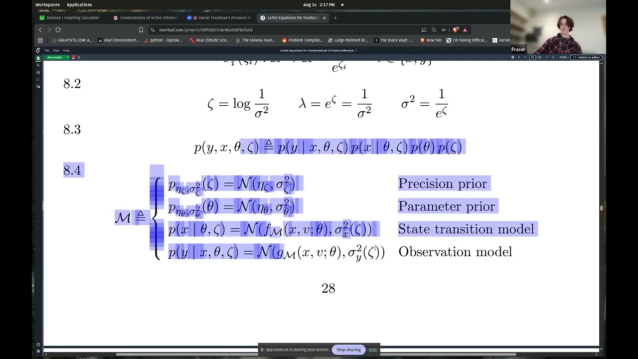Uh so perhaps if we go to 8.4, this is just a list of all the equations. Basically, this is kind of what our model is going to end up looking like. Something like this. So I've I've skipped ahead just very slightly. The idea is that well what have we got? We've got our our um prior on on state transitions. We have our state transition model. We have our observation likelihood given by our observation trans observation function. And the state transition model and observation function they not only take the hidden state they also take this um uh autonomous state as well that's going to be sort of driving the dynamics in some sense or rather an exogenous state and then we also have our variances on both of these beliefs and they're all Gaussian they're all bell-shaped curve now what is this precision so we've got prior now on our model so we have prior on the the actual parameter whatever those are and we also have this other kind of parameter the precision all right and we have we have a belief we have a prior about precision and a prior about the parameters themselves key I've just taken these these have been taken from from the text the thing is precisions of course this is the inverse of the variance of our model and we must keep in mind that throughout this entire chapter we're still in um the realm of uh the the uh the LLAS approximation or quadratic approximation where we're saying the the variational belief is very tightly clustered about mean. We only really have to care about the mean and then we're we're fine swirl and dandy. So the the thing the thing with precisions is that they have to be positive. They must be positive. Okay, you can't have a precision that's negative. It can be zero in which case that's kind of a a degenerate case. But we must make sure that our precisions are positive. So he introduces this is equation 8.1 a bit of a transformation where he says look well let's take the variance okay uh or or precision we need to make sure that this is positive how can we do that well we can take a transformation called the logarithm and that will make sure that um when we exponentiate that we can get back something that's positive. So that's this is really just a trick to make sure that the variances at issue are are strictly positive well or zero. Um and this is so what we're really dealing with is we're dealing with log precision. So the precision is the inverse of the variance one over sigma squ. Take the log of that you've got a log precision. And very handily uh the log precisions are donated with Greek letter zeta. Okay? It looks like a weird squiggle. It's almost impossible to write by hand. So these zeta things, these are log precisions. That's what they are. And how do you get back your regular old precision from this? Well, you just exponentiate the log precision and then you'll get that. So, really quickly, let's look at a graph of just yals x, right? That's just that's my precision in some sense. If I take the log of that looks something like this. All right. Uh, conversely, the exponential of a precision or some y= x looks like this thing. So in some sense you can kind of see colloquially that the the exponential and the logarithm they're kind of familiar images of one another. And indeed if I take the exponential of the log of x so log you know x is just my purple line. Exponential of the log of x I get this green line. And hey presto that is x. Okay. So the only real thing you need to take away is that log and exponential they kind of undo each other. And that's all we're really doing here. So we got log precisions. Very nice. Our model now is going to be it's going to sort of be enlarged. So not only you know we have our joint probability distribution over observations hidden states parameters and now also log precisions. Okay. And we're going to assume that they factoriize in this manner here that allows us then to spin off this the the version of the model that we have. Um, and it's a little bit obscure here, but we have a precision for the state transition and we also have a precision for the observation uh model as well. So those should really be like z and zeta x and zeta y. Okay. All right. So that's what we have. We've enlarged our model. That's basically what we've done. We've just sort of in we've we have a a larger space of things that we're now considering beliefs about. uh one very helpful thing that's it's on the it's in the text here. So of course we're we're we're dealing with the LLAS approximation. Okay, so we you know we have a joint uh approximate posterior now over these things or rather over these things. Okay, that's going to introduce a bit of difficulty for us. So, we now need to let's let's think about what the the variational free energy would look like given this new model of ours. All right. Um well, we can sort of under the LLAS approximation treat the variational free energy as equal to the negative log probability of of our generative model. Okay. So, we can just substitute stuff in and get all right. Well, negative log of our generative model properties of the factorization, properties of logs, we get this expression here. Very nice. Uh, and then we can substitute in the specific forms of the of the densities at issue. Um, and then crucially we have prediction errors. And just like we did in in chapter six and seven, we have our observation prediction errors. We have our well crucially from seven, we have our hidden state prediction errors. And now we also have parameter prediction errors and precision prediction errors. Um and if we if we ignore certain constants that come up given the lelass approximation, we can express the variational free energy much as the same way we did in chapter five and six as the sum of these precision weighted prediction errors. So we have our precision weighted prediction error on observations, hidden states, parameters and now precisions as well. Uh technically there is a there's an additional kind of log precision term in each of these prediction errors here. um you can kind of ignore that under certain assumptions. Um and that's a simplifying assumption basically. So maybe it would be more helpful if I went back to let's go to the actual notes themselves. Okay. Yep. Section 8.1. Perfect. Okay. Yes. Yes. Yes. We do a log transform. Very good. Very good. Okay, so that end we end up with equation 810 which is just uh we have our precision weighted prediction errors. Okay, and again this is really the same machinery we've seen from from chapter six and seven. Um it's just that we have an enlarged set of things that we're we're considering now basically. So the really there's and there's of course some discussion about it relation to predictive coding because it's very very similar looks looks very similar. The main kind of thing the main uh idea of chapter 8 is really 8.1.2 I would say uh basically this is kind of the the whole this is where you this is where the whole thing would hang together. So what have we done? We've enlarged our model. We have beliefs over hidden states. We have beliefs over uh precisions and we have beliefs over model parameters. And here's this is very nicely put on on chap on page 183. So update rules for learning and attention. Essentially we have kind of three different things that are changing. Um as I say the hidden states they're changing really quickly from from you know second to second or maybe millisecond to millisecond. And you know that's the whole the story about inferring hidden states is the story of just Beijian inference more generally. Okay, so we've seen this all the way back in chapter 2. That's where we started. You know, we're inferring hidden states and they they're changing relatively quickly as observations come in, right? But now we have these precisions, okay? And those are kind of the width of the beliefs at issue. And the idea is that well these are changing as well, but they're not changing quite as fast as the hidden states themselves. um and but nevertheless we have beliefs about them. Okay, so we we're we're seeing that there's a separation of time scale now. Okay, so we got fast changing stuff here, slightly slower changing stuff here. And if we think about it colloquially, I don't have um uh I don't have a nice figure, but obviously, you know, we're we're looking at Gaussian beliefs. Here's a nice figure. So, you know, this red belief over here, this is kind of more spread out than the green one. It's less precise. It's got more variance than the green one. We've seen this a lot. And at least in a colloquial sense, this is motivated what we can interpret what this means as the precision encoding, the degree of attention that one would give uh to um the the hidden stated issue or at least how strongly it would be updated. So if I go back here, whoops, no, I want to go back here. the these positions are going to be likened to and indeed there is a lot of discussion around how they are relevant to attention. Okay, so there's hidden states. They're changing. I've got beliefs about them, but you know, I should probably attend to hidden states that are very precise. That's that's the the second sort of time scale. And then again, sort of colloquially at a slightly slower changing time scale, we have the beliefs about the model parameters themselves and we've seen their connection to learning. Okay, so we've got these three time scales. What this does is it introduces a bit of a problem. Okay, so I've got my perception, attention, and learning uh there. We have a belief about the joint uh state now. Okay, so we've got the hidden states, precisions, and parameters. So our our approximate posterior is going to have to range over all of them. And there's a question about how we can do this. um what should our approximate posterior belief look like? There's all kinds of interesting um answers to that. One answer, one very kind of simplifying assumption is that we can say well my belief about the joint state hidden states, precisions and and parameters can be broken down into the product of belief about hidden state times belief about precision times belief about um model parameters and that's called the mean field factorization assumption. Okay. So this is this is saying I believe that hidden states or you know my my my joint belief about all of this these combined hidden states breaks down into the product of the the individual ones. Okay. Now that may or may not be true in the generative model. Okay. Um but it's a simplifying assumption and it helps simplify the maths. We don't actually need to make this assumption for generalized filtering. uh but it is it's nevertheless an important assumption that is made in in certain other um places. It can be made here as well. So it bears commenting on. Okay. So yeah, we shouldn't claim that the mean field assumption uh means that the variables have no relationship to each other in the generative model. Uh it's really an assumption about what we think our posterior belief is like. Okay. Uh they can still be coupled. So you know x can still be coupled to theta can still be coupled to zeta indirectly. Um that's yeah so just a little bit of a clarification. Okay now problem we know that if we're going to do hidden state inference we need to minimize the variational free energy okay or the precision and we're going to operationalize the variational free energy as precision weight prediction error. But that's only accounting for one part of the combined hidden state belief now. Okay, we've got hidden states, precisions, and um parameters, and they're all changing at different time scales. So, this seems like a a real problem. And the way that we're going to kind of solve this problem is we introduce rather than considering the variational free energy kind of, you know, at each point in time instantaneously, we're going to consider the kind of accumulation of the variational energy across time basically. So from now you know sum it up for however long we happen to be going for. And this thing has a name. Uh it's called rather unhelpfully the free action. So it's the sum or in this case the integral of the variational free energy across time. And this thing is going to allow us to capture all of the kind of temporal dynamics at issue. So it's we're going to have the hidden state transitions precisions and parameters be able to be represented in this formalism. The idea is that this this other quantity called the the free action. This is kind of the fundamental thing. Now it's the the sum of the integral of the variational free energy. Very important point. Uh free action. So this we're calling this thing an action. This is completely distinct from what an action is uh given by the the agent. So the agent emits actions, right? And it receives observations. Uh this is completely different. The free action has nothing to do with action in that sense. where it comes from the name you know free reaction this comes from a branch of physics um Hamiltonian and lrangeian dynamics but they're completely different things don't don't mix those two concepts up very important all right now so we've got the free action we've got an enlarged model we have a state space that's ranging over kind of three canonicalish time scales um how are we going to do the story of minimizing variational for energy or in this case the free action across time how we going to do inference learning and attention. That's that's the story. The crucial thing is to understand that well look the variational free energy. Uh if I if I take the derivative this is just a fact from calculus. If I take the derivative of the free action cross time that's going to cancel the integral and I just get the variational free energy back. So the variational free energy is the derivative of the free action cross time. Excellent. And I know how to minimize variational free energy. We've done that in chapter seven and six. So now we can start to think about how to operationalize what we're doing in our combined model. Yeah. So VF is an instantaneous objective. Free action integrates that objective over time, you know, given some path is the idea. Uh caveat caveat. So uh well we want to do gradient descent on the variational free energy. Um and we can do that by means of talking about how it you know its relation to the to the free action. So this is on page uh 184. We can talk about the motion of our belief about parameters. We can define that as the gradient or the negative gradient in this case of the free action with respect to the parameter at issue. So we can do that for parameters and precisions. And this tells us how the uh the parameters and the precision beliefs are going to change across time. And of course we have a negative here because we want to go down the variational free energy gradient or down the the path of least action. Um now if we take uh the time derivative of these of this and then also of this we we end up with things that look a little bit more familiar now. So we have our acceleration. So this mu double dot is saying take this is the rate of change of the rate of change of our belief about theta. Okay, it's an acceleration. So we got position, velocity and we've got acceleration, right? This is the negative uh well the gradient of the variation for energy with respect to the parameter and then also we have the same thing for precisions. Excellent. Except now h well this is a second order differential equation. Okay, so we saw the first order differential equation in in last chapter. This is a second order differential equation. Mu double dot, right? How are we going to solve this? Well, that's there's there's a trick that you can use, not really a trick that will turn a second order differential equation into a first order one. So I I go through here and I talk about that trick and I kind of motivate it. I give a nice sort of well what I think is a nice mechanical or physical intuition that basically if you've got any kind of second order differential equation you can introduce a completely new variable and say well in this case let's just say I've got q dot is some function I can just introduce a new variable r and I can define that equal to the first derivative of q and then if I take the derivative uh well and that gives you the first derivative of q if I take the derivative of r that gives me my second derivative back. So now I really only have to talk about r and r dot and those are first order things. So you can end up decomposing the second order differential equation into a system of coupled first order differential equations and then we can use oilers's update rule and we can do everything as we did before. That's the idea. So sorry for um covering an entire semester of differential equations almost in about 30 seconds. Uh that's the sort of situation we're in. So I give a few examples about how to do that and then I say okay well how are we going to apply it to our specific case here right? So we we have our second order differential equations. We don't want to that's too complicated. We want to turn them into first order differential equations. So we just introduce a completely new parameter mu prime theta and we define that equal to the first derivative of mu theta um and then we can take the derivative of mu prime theta and that's going to give us mu prime prime theta lots of bookkeeping and then we can do the same thing for the belief about precisions as well. So then ah very nice we can turn our second order differential equation into a couple first order differential equation and and we can use oilers's update rule that's that's all fine we can do the same thing for the precisions as well so now one further little modification so that's equation this is literally from the book this is equations 8.16A for the motion of the belief about hidden uh parameters and also for the motion of the belief about precisions Uh, excellent. There's one further modification that Sanjie makes. Um, and then 8.17 A and B are he just gives you you can substitute these back into the to the gradient of the variational free energy and get a precision weighted prediction error. Okay, that's that's standard. The um he introduces one further little modification this dampening term. So you know 8.16 a and b they do a little bit more than just rewrite the second order differential equation. Um the idea is that we're going to also in addition to mu prime we're going to introduce we're going to basically say we want mu uh prime plus a damped version of it. Um, the reason for that is that it's it's going to make uh the the the integration of the system a little bit easier to deal with. I explain it here kind of where where that comes from, why we're even doing this. Um, it is a nice modification to make, but I wouldn't spend too long worrying about it. So, this this is kind of the assumption we're making. So you know the acceleration of the parameter belief plus a small amount of the the velocity of the parameter belief is going to be equal to the negative gradient of various energy with respect to the parameter belief. Oh my lord that is a lot of stuff to uh to keep in in one's head. But if we can do this and we can do this, we now have a way of formalizing the whole problem um in terms of the the gradient descent on variation for energy and we we we've sort of seen that story from chapter 7. So now we can actually do the inference uh learning and attention all at the same time. So I go through and I give a mechanical analogy for for like a physical system as well talking about you know where this comes from and I give a a loose correspondence between the variational story we're telling with respect to beliefs uh or sorry over here and then the this the physical story with respect to maybe a ball moving in a in a whale or something like that. So that gives a little bit more context as to where that kind of ma mathematical machinery comes from. That's not in the book. Um that's kind of the purpose of these notes. Uh yes. So yeah, why why do we care so much about turning the second order differential equation into a couple first order ones? The idea is because we want to use Oilers's rule. Um first order differential equations are easier to to actually kind of compute numerically. Um so that's why basically it's for practical reasons essentially. That explains that there. Okay. Excellent. So at the end of this we have our our VF gradient. This is 8.17 uh a this one here. So much as we did before. So we have our precision weighted prediction errors on uh hidden state transitions and then also on observations. And so this is this is the gradient of VF with respect to the belief about parameters. We can do the same thing for hidden state uh precisions as well. Now, all right. So, we got kind of three copies of the same thing we've seen floating around. You know, gradients of VF with respect to hidden states, with respect to parameters, with respect to precisions. We're going to collect them all together now basically into so and to you know, we can say all right good. What's the motion of my approximate belief across time? What's the motion of my variational posterior belief across time? Well, my variational posterior belief is made about it's made up of my belief about hidden states, belief about parameters, belief about precisions, and the two other auxiliary things that we added um relating to the dampening terms for the conversion of the second order differential equation into a couple first order ones. And we have expressions for all of these things. So that's you know we can just substitute that in and we can say look the the motion of my belief overall is equal to this thing here and we can calculate all of this stuff which is very very excellent for us and again the thing that I would want you to come away with is that we have a story about how perception happens how learning happens and how attention happens now and they they they happen over three different time scales. So we got kind of fast changing stuff uh relatively slower changing stuff and then slowest changing stuff basically and it's the use of this free action or the the accumulation of the variational free energy across time that allows us to tell this story now and this this is this is going to unify the stories of you know perception action sorry perception tension and learning that we've seen before. Uh very good. So you can you can do the oil updates now um no problem. So you can do them with respect to the the beliefs at issue and this culminates in algorithm 12 which is the generalized filtering perception sorry the generalized filtering algorithm for perception learning and attention. So it's much more it's much nicely much more nicely type set in the book itself. This is just a sort of huristic overview. Um I think we might have a a picture of it that might be nice. algorithm 12 maybe not okay anyway so I put it there for for reference so then finally enough enough theory we actually get to an example we go to example 8.1 uh so so 8.20 20 is the equation at issue and we're going to say all right well how do we do this for you know learning first and second order parameters for you know in in the generalized uh case basically well actually this this is just a univer case um but we want to do generalized filtering in the univariant case for a really simple model and this is the model we're going to consider extremely simple um state transition dynamics and observation um generation. So this is the this is the generative process specification. The generative model now has as before observation likelihood um state transition well uh prior on on state beliefs and that's given by state transition function. Crucially in this example um the observation variance is fixed across time. So you see you know the the precision for hidden state the hidden state prime that's not fixed okay we do have a belief about it but we don't have a belief about the observation precision that's just sort of fixed and given at least for this example just to make things simp simpler and then uh so that's our model if we run that we get figure 8.2 too, which is much more exciting to look at than equations. All right, so this is the results of of um this example. I would strongly encourage people to try and implement this example. I'm going to try and do that myself hopefully in in preparation for next week. Um but we can maybe talk about it. So this this at least gives you the the core, you know, of um what we're talking about here. So we have our we have our belief about hidden states and we have the hidden state. The hidden state is in is in gray. Okay. And that starts out way down here. Okay. And the belief starts out way up here. So there's quite a quite a mismatch, but across time we see that they very quickly converge. Uh as well as the observation and predicted observations, uh they start out fairly all over the place. And the variational free energy on on the right, this almost immediately collapses to extremely small and stays there across time. But and and okay, so that top row that's effectively chapter six kind of basically um and we're not even really doing any action here either. So you know it's kind of standard chapter six. The additional thing is we we also have beliefs about the parameters and the precisions across time. So the idea is that all right we can see that these actually do end up converging to you know values that are very similar to what they should be. So the actual theta here is uh what is it three that's right observation likelihood theta is three so we end up converging to three across time um and the precision is I think it's set to one is that right a very very small uh it's a bit hard to see on this this plot and then we have the prediction errors as well I think there's a bit of a mismatch for the um notation we've got you know epsilon h and epsilon Um I think that should be epsilon theta and epsilon zeta which would be very fun to say 10 times fast. So I I think example 8.1 that's kind of the central example for getting all of the motivation that and you know conceptual grammar about what's going on what we just did at all. So that uses that implements the story of you know variational free energy minimization with this free action thing with an enlarged model and we have beliefs about the parameters and the the precisions. Now now that takes us to 8.2 hierarchical forms and this is really exciting. Um however just quick stop for questions. Are there any questions at this point? I want to go through chapter eight well you know section 8.2 and then we'll open it up for more questions. But are there any questions at this point? I don't want to just scream into the void if people are keen uh to ask for clarification. >> Just a quick comment about figure 8.2 that epsilon H and epsilon G. The HG comes from the um SPM DM toolbox from Carl Fristen where they use um the H stands for hyperparameters and G stands for something related. So that that literally maps in our case to the um attention and uh learning uh >> okay that thank you for thank you Kobus that makes sense. I was I wasn't sure where that came from if that was just an earlier code um uh transcription but um okay that that's that's no problem there. So and as I say hopefully so you know for chapter 7 I put this is for from last week now I put the um example the the collab example of you know univari active inference for the Bayian thermostat up um I would recommend copying this and then you can play around with it yourself. I would like to do the same thing for example 8.1 at the very least because that's that's a I think that's a crucial example to study. So if you really if you want to kind of grock this chapter and understand what's going on 8.1 is is where you want to go. So back to chapter 8. All right I will press on with uh you know uh section 8.2. Now this is a really really cool section. Um lots of very interesting ideas are coming up here and ideas that we'll sort of see again. Also ideas we've seen before in in chapter five. So the the main idea if we go back to some notes hopefully it's not too depressing to look at all of these these notes I have back. All right, the main idea now is we want to we want to uh be able to tell this story about inference in our enlarged model where we're considering um hidden states, precisions and parameters in a hierarchical setting um not just univariatic. Okay, that's going to that's going to give us the the most bang for our buck. So rather than immediately going into equations the we consider that he starts out by considering the simplest possible case. So figure 8.3 is somewhere 8.3 1.2.5. Oh it's not there. I'll set it. Is that right? Yeah. So you know he wants to show you a Bayian network that looks at the the simplest possible example. Sorry, I thought we had it up there, but uh we don't just now. So, you know, I I do start out with a kind of big picture overview here. So, the thing is we can think about what we did in 8.1 as specifying a generative model that is kind of like one layer and we're going to be able to stack these layers on top of each other to get a more powerful generative model. That's the idea for 8.2 basically. So I do recommend figure 8.3 having a look at that. Um essentially if we go to what we're going to have to assume maybe I have a I don't really do that. Okay. All right. Doesn't matter. Basically the change we're making is we're assuming this is the same sort of structure that we saw before but we're going to assume that these are multivariate now. Okay. So our our observations are multivaried our hidden states exogenous force or exogenous state parameters and precisions. That's the kind of big thing that uh we're assuming now. So the actual structure of the model is going to look almost identical. Um we have so we have you know beliefs or rather prior about the precisions the uh parameters also the autonomous states they're going to have a prior now and it's much more illustrative to we do have exam uh figure 8.4 so let's actually look at this in 8.4 for so what's going on? Uh this this is the um uh what do you call a Bayian network view picture of the model. So if we look at on the left um this is now for a dynamic generative model for obviously we're considering hidden states changing across time and they're multivariate. So things in bold the x the v sigma well okay yx v in bold these are vectors these are multivariate things now so circles denote random variables so x is something we're uncertain about so we have a belief about it gets a circle right and the belief is the state transition belief right up here uh parameterized by the mean being the state transition function and the co-variance being dependent on our precision Um, and so that affects X. The autonomous state affects X. Theta affects X. And X generates observations. So Y are our observations. And Y is kind of shaded in gray because it's something we can observe. Uh we we're we're only allowed to observe things shaded in gray. So things that are white, we're not allowed to observe. We have beliefs about them. Um nevertheless, we have beliefs about how observations are generated. And that's given our observation uh mapping belief. So that's great. Um, and of course basically chapter 7 sort of dealt with this picture where we had um an autonomous state affecting the the transitions in our in our actual hidden states. But we we can now we can now have beliefs about the autonomous state as well. So that's what I showed you in terms of the model. So 8.23 two three. We can enlarge this picture now where you know so we have our generative model over observations and hidden states factorized as an observation likelihood and a prime over hidden states that's been the same all the way through since chapter 2. Same sort of thing again except now we can include an additional belief about these autonomous states themselves uh and we can update our belief about them. So that's going to give us a bit more power basically in terms of what we can reason about in our model. And that just shows up as another um another factor in our model. So we're going to have our model factorized like this now. So again it's it's a random variable. So and it's unobserved. So it's a it's a node and it's not shaded in. Um and but it's parameterized in terms of other stuff now. So it has a mean and that means going to be this at V. Uh and it also has a precision that's parameterized by some some precision and those are just going to be fixeds. Okay. Yeah. So, that's going to get us to I want to go back to my notes. That gets us to figure 8.5 which is like the the atomic unit of what we're dealing with basically. Adding hidden state prior. Yes, we talked about that. Yes. So, you know, we talk about making the autonomous state probabilistic. We have a belief about the autonomous state now given by some in this case fixed ATA and well not fixed the precision about uh the autonomous state. So really the only difference is that we have this belief about the autonomous state in here. Now basically that's kind of the only difference. Um do I want to talk about that? No not necessarily. There there's a bit of a talk about multivariate log precisions and covariances. So the idea is that okay in the multivariate case we don't have variances or precisions. We have covariances and precision matrices. Now so really there's just a a transformation that goes through that. If you're unsure about that I' I'd have a look at chap um appendix C that goes through more the notation. We don't need to be bogged down by that too much though. Um okay so really what do we end up with? We end up with this figure 8.5. Haha, perfect. This is an extremely important figure to understand. So this is the Beijian network for the full dynamic generative model with prior on parameters. So we have a prior belief on parameters now. So that that wasn't a circle before. Now it is. We have a belief about it. And that is itself parameterized by some ATA theta some sigma theta. Okay. We have beliefs about parameters. We have beliefs about precisions. Where are those? They're given here. This should really be I'm not sure if that gamma should be a zeta. I think it should be. I think that might be an RA. What do you think, Kobas? Do you Because we we used the gamma before. I think that should actually be a zeta. >> Yeah, I agree. I I prefer it to be a zeta as well. >> Yeah. Okay. I think that's we'll have to note that as an arata. So, we have a belief about our well, in this case, log precision. I should be careful. So zeta is a log precision. Okay, we have beliefs about autonomous states. We have beliefs about hidden states. So this entire slice up here, this is kind of what I've been talking about this whole time. And of course, hidden states give rise to observations. This whole thing, so our model, it looks like this. And all of so you know, observations, hidden states, parameters, precisions, these are multivariants. You know, they're more than just one thing. Um these are this is our model. This is our generative model for the dynamic case. This is this is kind of the atomic atomic unit. Um what we're going to do is we're going to stack these on top of each other to get a hierarchical generative model. And that's going to allow us to do lots of very powerful things. Really quickly because I do want to leave a little bit of time for questions. What you can do is you can go through and do almost exactly the same maths that we did. So 8.25 25. You end up being able to say well the free energy is the sum of the squared precision squared uh precision weighted prediction errors with respect to observations uh hidden states autonomous autonomous yes autonomous states uh parameters and precisions you can spin up expressions for the prediction errors with respect to observations and hidden states. Obviously our observation function is now a function of hidden states and the autonomous state and the same for the the transition function. You can do the same for prediction errors with respect to the autonomous states parameters precisions and then you can do that story where we get the motion of the hidden state is equal to um this big old vector here in terms of the variational free energy. Okay, excellent. Perfect. Now the really exciting bit is where we go into making this hierarchical 8.2 2.2. Um, fundamentally, this is the idea. So, figure 8.6. Yes, perfect. This is what we're going to do. We're going to take copies of our model and we're going to stack them on top of one another effectively. And you know the reason why we might want to do this is because this allows us to represent prior or beliefs about how things are generated in a way that is going to be more powerful than we can if we don't have this hierarchical situation. So this is we're saying this if we this is just two layers. If we look at one just the bottom layer here, what this is saying uh is that my belief about how hidden states are generated is that there's some autonomous state, there's some parameters, there's some precisions, they combine somehow and that generates a hidden state and hidden states generate observations. But this whole thing if we consider another layer on top of this corresponds to a different set of assumptions. It corresponds to my assumption that the autonomous state is itself given by some pro some hidden state that is parameterized by parameters another autonomous state and more precision. So we can kind of keep going with as much as we care to in in this this process here and then we can just say well look the whole generative model this is very much as we had before except now it factorizes across these layers. Okay so the very bottom layer L equals Z. So we've got L little L going from zero to big L at the very bottom layer. This is actually this is this is a typo. This should be Y the observations Y. Okay, we we do literally observe something at the very bottom layer. Uh but then as we go up in the layers, so we got layer one, layer two, this autonomous state is going to kind of in some sense play the role of observations uh for the layer above. That's that's important. there's there's lots of um uh I would say there's an important detail to to not be confused by in terms of the direction of the the generative direction. So, you know, my generative model is making predictions about observations. That's one way. But when we're updating our model, we're going from the bottom all the way up to the top. So, I spend a bit of time in the notes here talking about that. Uh I don't want to necessarily go over it too much. Uh so we got layer wise probability distributions uh yeah two directions in the hierarchy generation and inference. So gener generating predictions that corresponds to me saying what observations do I think I will get conditioned on a belief about the hidden state right that's kind of my observation likelihood and then inference is well I get an observation in uh what hidden state do I think caused that okay these are two different directions and it's important not to confuse those directions um the layers here these are sort of indexing the the generative direction okay going down from the very top to the bottom And then when you go up that's inference. Uh and it's important it's also important uh to not confuse those two things. It's just reversing the arrows. There's there's different processes that are happening but they're coupled across layers. And the way that they are coupled um I'm just scrolling through here to give you a sense of the fact that there's a lot more to be to be talked about about that. The way that they're coupled is through the autonomous states uh 8.6. You can see you know I plug in one by taking the auto state of another plugging it into the bottom one. So that is the end of 8.1 and 8.2 and I would say the fundamental machinery of chapter 8. Um 8.3 to 8.6 is really just kind of extensions and and different flavors of things. There's lots of very interesting connections between this idea and portical microcircuits in the brain. I'm sure that Andrew can speak to that a little bit more than I can. Let's come back to to here just now. Uh yes, Andrew, excellent time for you to uh to share any any thoughts or anything. >> Yeah, thanks. Uh you know, very good, very nice uh lecture. I rose my my hand earlier, but I didn't want to interject because >> Well, no, no, no. Just uh my question is is something that's more general about this chapter and honestly probably shouldn't really come up too much until next week whenever we've kind of worked through the rest of the chapter. But uh yeah this uh this matter of like hierarchical models which were already introduced uh to the notion of hierarchical models back in in chapter 5 on predictive coding. Um so here it's it's just kind of interesting and a bit tricky to talk about hierarchical models in that in chapter 8 uh in the earlier sections it seems where we're the way we're introduced to them is sort of like um you know your sensory observations your why is as if it's at the lowest layer and then above that at another layer are the hidden state and uh and and autonomous states V. Um whereas later in the chapter as well as in how hierarchal models are um introduced in predictive coding um an a different way of conceiving of these layers is actually the lowest layer contains your why as well as your hidden states and your autonomous states. And then the next level up would be, you know, a similar sort of construction of something more or less along those lines aside from we'd be swapping out the the Y for the V from below or perhaps in states from below as well. So it can get a bit tricky just um in this general sense of the way we're introduced to hierarchical models in this chapter is that like sort of within a layer you can kind of conceive of it as having its own uh sub layers with the lowest layer being your why your sensory observations and the next layer up in the states. So I just wanted to point that out um that that that it can and >> uh the part of hierarchical models is is that it it it's becomes perspectival sort of in a certain way kind of depends on how you're yeah looking at it. And furthermore, I mean, you know, aside from this notion of there being sort of ascending predictions and excuse me, ascending uh prediction errors and descending predictions, um hierarchical doesn't necessarily mean you have to always think of it as from the bottom to the top. Like as we see later in the chapter on all these things about message passing like you could have rather arbitrary constructions where you have what seems to be a lowest layer but actually it's you know you could have these sort of lateral connections other layers and the rest. Um it can be very fun but also a bit daunting to to think uh all of it through. Um but but yeah, so I just wanted to um yeah, point that out. And then again, uh later in the chapter is probably where some things might get clarified, but uh more generally um it's in this chapter that we see the most on um message passing. We get much more detail about these sorts of kind of network and graph type illustrations we've been seeing in the textbook. So um yeah very >> quite visual very handy. Yeah. >> Yeah. Absolutely. I think it's very worthwhile for for readers to um get a sense of for those who are new to these kinds of things because many of the illustrations we've seen so far like typically the the the caption will say like a basian network which is one way of conceiving of of these kinds of probabilistical models as probabilistic models as graphs. Um but then there are other kinds of you know graphical structures that we could use and there are fory factor graphs and the rest with their own respective terminology. So it's worthwhile to spend just a little bit of time thinking uh with with graphs. You know there will be many people who are familiar with basian statistics and the like but they're not used to saying these sorts of like relatively complex graphical structures. Um and so just being familiar with like what is a node you know what is an edge? um those sorts of things. Um oh and yeah, thanks for uh bringing up the slides. I tried to give a little bit of that in a couple new slides I I added. Um this is just, you know, we see triple estimation where we've now introduced attention. Uh and then yeah, more on the the way that we're conceiving of sort of these error units and state units and all things that kind of uh succeed uh section 8.2. So probably next week sort of level material. Um and then uh there's a an attempt to explain algorithm 13 which is definitely a end of chapter kind of thing but I wanted to have some yeah just a sense of this is sort of what we're all building up towards. is like we have the hierarchical attention precision uh modulation and and we have learning and we have action we have so so algorithm 13 is a really nice way to um round off all of this fundamental material we've been seeing on continuous state space models um I think we're about out of time and we have a whole another round of lecture next week so I'll stop there but I I think it was very important the way that you covered uh all these fundamental that we're getting into and thinking about uh layers and and the hierarchies, thinking in terms of graphs. Um being able to understand the relationship between sort of uh V and sort of where it it sits in all of this since we know that V is uh new. That's the that's one of the newer parts aside from attention um you know in these past couple chapters. So yeah, thanks. >> Yeah. No, thank thanks thanks for that. And I I I must I didn't you did in in your in your slides, but um that problem is called the triple estimation problem because we're estimating three things. >> So that's an important thing. Yeah. >> All right. Well, I look I mean if there's any last questions for the recording, um that would be excellent. But I I might stop the recording here if no one no one does and then they can ask questions um otherwise. So going once, going twice. Vera, please. I don't know if it's actually for the recording, but uh if uh so what I really liked is that um this hierarchical um uh sense of um okay there's a the different temporal affordances >> aren't actually an implementation detail but they determine what counts as perception, learning and attention. in the first place and actually without those time scale separation those categories uh would collapse into just the same operation I guess and um so my question is if perception learning and precision precision learning all minimize the same variational free energy objective but operate on different time scales. What determ minds which level absorbs a p persistent prediction error or yeah I don't know or in other words um >> when does an error remain a perceptual update and when does accumulated error become evidence that the model parameters or precision themselves should change? That's my question. >> Excellent question. Yeah, I mean uh I think Andrew will have stuff to say on that there. But really quickly um if we just go to the to figure 8.6, this is not answering that question. Okay, so this notion of hierarchy um we might imagine that there are different hidden states and they change according to different time scales blah blah blah. We could imagine that. That's kind of what this is getting at. But your question is about well when does the belief about this versus this versus this versus this get updated. Um and there are that's that is quite a deep question. Um we basically we've only really seen a hint of that in the in the sort of framing of this whole process um with respect to the free action. So the the key the thing that sort of allows you to talk about all of these time scales is the free action the the accumulation across time of the variational free energy. I did have it here. Um so yeah like when exactly you should update your belief about um hidden states as opposed to parameters. This is it's it is a bit of an uncertain question although in in certain you know biological applications it can be it can be a little bit clearer or you you you have some principled way of thinking about when you should do that. So there's actually been a lot of work in isocarts. So uh so this is you know where are you sort of looking uh your your gaze you know you can decide to attend to certain things but then your eye is while you're doing that performing these very very small fine motor motions that are that are trying to resolve uncertainty at a at a much smaller layer. Um so exactly you know and that's that's at the level of sort of milliseconds your your gaze is at the level of maybe seconds. So there's if you wanted to model that process there's at least some empirical separation but determining the causal and structural reasons why is is is an open question. Um, I'm actually less competent about answering that question myself other than other than to say that there are, you know, principled um, examples from from biology that can that can help answer that. So, I don't know if if Andrew you had anything to say on that specifically. >> Yeah, thanks. I uh yeah I mean it's a it's a tricky question uh and and I want to make sure that I'm understanding it well enough but um because I I mean I if you remove the time the temporal separation if you remove the time scale separation then sure you still have if you're still using the same uh sort of equations um it depends on how we want to conceive of the time scales the the time scale separation can be because you wrote your algorithm to only have particular things update, you know, every other time step rather than every time step. Like you could have parameters updating, you know, every second time step whereas in states uh, you know, update every first time step or you could have some other arbitrary set of rules here in the continuous example that we're getting in chapter 8. It's a little bit less about doing that sort of thing and it's more about the way that we're treating these first and second order parameters. The way that we're applying these different temporal derivatives to where you know if we apply uh if we include additional ones for parameters that allow us to have this sense of uh even further change over time to where there is this sort of uh conceptual like slower time scale that they're operating at. assumptions sort of baked into how we're applying those um derivatives and including them in our model. You know, that that's all fine. But but um >> so so that I mean you know with the time scale separation a lot of that is just drawing from sort of empirical studies of of the brain and information processing and and you know all these phrases of recogni recognition dynamics that themselves precede specifically active inference. uh that it's a much broader term uh just as you know basian uh statistics goes much further back um but with respect to uh prediction error and and minimizing free energy I mean a lot of um where that sort of settles is really going to to depend on the actual simulation at hand right because if you have um you know if you have a relatively predictable uh environment where there are no sort of regime changes is at any point where the the the the the environment becomes like virtually, you know, different like the world's very different whenever it's raining, right? Like many things can or let's say storming outside, you know, maybe there's some awful storm going on outside and suddenly stores are closed and no one is on the street and there's a lot of danger for people to walk around versus whenever it's not storming. Like that's it's a very different kind of environment to navigate, right? So you do need that um you know ability to like you know almost confront a a very different world. But if you had a relatively static world uh that that you know perhaps it has certain kinds of of rhythms in it that need to be attended to that you know you do need this sense of temporal derivatives uh in there to be able to catch things that that change and catch the sorts of patterns that are going on but it's still relatively static. you would very frequently ideally see very low uh variational free energy. You'd see very low prediction errors assuming you have a good model. Um whereas if you have uh an environment that like drastically changes that calls for different sets of actions and different kinds of hidden state inferences and very different observations elicited from the environment in sort of one regime or another. Then you'll see prediction errors very often very reasonably, right? Because it's it's the prediction errors themselves sort of motivate an agent to adapt or change its sort of behavioral behavior or the way that it updates uh you know V for itself so to speak so that it can adapt to those changes. So I I hate that my answer is really just it depends on the circumstance at hand. Um, and what I sort of got from the question is, you know, I I I say all this because it's important to remember that prediction errors are not necessarily uh, you know, them in and of themselves like bad or or exemplify a bad model. like a a model that's able to use prediction errors to its advantage to properly learn uh is in some ways qualitatively a better model than say a standard forward model that you know maybe it has prediction error but it's like oh I'm you know in in plainst terms a simple model that says oh I messed up I'll do better next time but there's no update to my parameters and there's no update to other things that need to be updated where I could use those prediction errors as and uncertainty as information for updating my model. So I I could kind of go on, but you'd see it's getting a little more conceptual. Um but I just I I hope that it's understood that the I I don't know if there's a very clear specific answer to that kind of question. It might be the way that it's being framed. >> Yeah. >> Yeah. Thank you. Thank Yeah. Sorry, Razer. >> Two things two things on that. Ver like just quickly chapter 8 doesn't purport to offer an answer as to like well when do I update my beliefs about precisions or parameters or hidden states it's just saying that these are there are three characteristic time scales and the updates are in some sense kind of given by the dynamics at issue um but you could absolutely decide or or you know intervene at c certain times as opposed to others um like okay well I want to update my precision you know every every single tick or something like that. That could be something you do. But chapter 8 is not trying to do that. It's just kind of showing us that it's possible to frame the question of inference more generally as this larger problem within which we can do, you know, free energy minimization to solve uh for beliefs across those time scales. But you could you could you could decide to intervene on on some specific time scale if you really wanted to. Um I put in the chat that question though about like okay well when when should I update as opposed to not that's very relevant to one extremely hot area of research in active inference now called structure learning um so there's a paper there by by Lance and a few other people um that's that's if you're interested in that question while they're like when should I update uh beliefs about hidden states versus parameters versus the structure of my model uh that that comes up there in that issue of structure learning. Cool. Thank you. But uh sorry to be so conceptual, but I think I got it. It's like just a question uh which part of the generative model um should be plastic and on what time scales. I think um yeah. >> Yeah. Yeah. And of course typically for a lot of interesting problems, it's precisely the fact that we have this hierarchical structure that's uh for a lot of problems that we want to be able to model things hierarchically. Um so we have that hierarchical structure but then we also have within a layer updates at certain times about you know precisions versus parameters versus hidden states. Absolutely. >> Also add on the Oh, sorry. >> Okay. Thanks. Uh yeah, on the the matter of which parts of the model should stay plastic, I mean it's also a good question also very going to be dependent upon the the situation at hand. I mean in some ways uh it would almost from one view it would almost be um you know beneficial to have literally everything be plastic to some degree and that's perhaps what's more empirical. Granted, maybe the way that that plasticity is employed in the model should maybe be aligned with different kinds of um empirical studies or otherwise using neuroiming looking at patterns and then think you know um basically like how in the same way that neuroscientists may have arrived at the idea of there being different time scales operating in the brain. Um you know based upon that sort of research perhaps whenever we apply a model we should be doing the same thing. But it's um you know if if you're going to employ you know a model that's just massive like the let's say we're in a purely computational space here. We're not concerned with empirical plausibility. We're not concerned with creating like an adaptive agent in an environment uh you know in any kind of um pseudo organic sense but rather something that's going to crunch a lot of numbers for us. uh you know some sort of stock price prediction problem or or or uh uh something along those lines. It's just going to the idea is that we'll be ingesting large amounts of data such that if we were to make every single piece of our model plastic that's going to mean that we're going to be implementing many many many update rules every single time step and we may not have the computational hardware necessary for running that kind of model. It might be in that case that you might start to sort of prune back the degree of prob probabilistic parameters in your model. You might say that we will have uh fa we'll have our parameters and precisions be purely deterministic and just static throughout everything and just hope that inference itself is what's able to catch and make better predictions from step to step. And then that way we can sort of reduce uh you know our computational hardware necessary for for the problem at hand. Um but yeah, it's it's sort of it's sort of there. It's it's going to sort of depend upon your domain you're working within essentially how much are you trying to capture empirical phenomena in relation to the brain and whenever I say the brain of course that's going to come back to which which brain are we modeling a human brain a mouse brain or the mamalian brain is generally there are many shared principles which is why uh some people will speak so broadly and why so much research with mice and the rest has informed human studies as well especially in cases where um the ethics would become more questionable if we're to carry out studies with with humans in certain circumstances as opposed to to mice. But um yeah, it's I I think I'm droning a bit. Sorry. So, I'll I'll just kind of leave it there. It it's still a good question, but it's going to come down to sort of your experimental design that you're employing and and your problem at hand. Yeah. >> Yeah. I'm just answering a few questions in the chat here that's been quite active. Uh so, there was there was a question by Jen Cuomo. Uh, is there a trade-off between changing parameters and minimizing VF sort of too much as it were becoming too rigid and more prone to failure and death? Um, I mean there's always the perennial problem of, you know, overfitting and underfitting, but the VF itself is meant to be this, you know, an approximation to a quantity that's telling you how well your model is doing at uh, sort of predicting or or separating itself from its environment. So I I'm not quite sure how to formalize this exactly, but it wouldn't be the case that you could minimize the VF too much. Um in the perfect case, you would have like zero um VF and you would be able to exactly approach the the log evidence uh bound and everything would be great. But um we obvious we can't do that for computational reasons. Um so it's not simply the case that like you can make it too small. uh although we have seen of late especially Andrew you mentioned this last time that it can be useful to have nonzero prediction error in some cases in the sense that this can give you useful information um so you know obviously the the precisions themselves these these are as we've seen these are likened to attention they can even be they might even be able to formalize what attention is so in that sense it can be useful to not always have zero prediction error But uh that's that is a that's quite a large um area in and of itself or a large sort of you know area of interpretation. So >> yeah. Yeah. It's it's it's so much of this is going to be highly dependent upon like well what is the environment that the agent is in? Um are all of the agents sensors uh so to speak that it actually has to receive sensory observations? Are they sort of all up to the task? Right? Um, you can also think of a scenario where that you have an agent who has uh, you know, it it it pays much more attention to sort of its priors on hidden states as opposed to updating them. Right? So, you could have um I'm sorry I come up with all these strange examples, but uh you know, if you if you were in the woods and uh you know there's a pretty aggressive bear running at you, um you could just sort of pretend that the bear isn't there. Like, oh no, I'm watching a movie right now. I'm okay. You know, and then if you were watching a movie of a bear, your model would say, "Oh, that's fine." Like, this is exactly what I'd expect. I'd expect, you know, bear in front of me because I expect a bear because that's what my prior say. I'm just, you know, convincing myself that I'm watching this movie. Now, we've brought VF way down. Like, that's great. Like, I'm going to survive this, of course, cuz it's just a movie. It fits my expectations of a movie. Um, but then you're not in a movie. So, then what will happen is that your VF will dramatically rise whenever, sorry, something something probably bad happens from there, right? That that doesn't align with being in a movie. So, so if you that's a very this is a very distinct rather violent uh uh uh example I came up with but but within the context of that like sure you could you could have a situation where VF was minimized uh you know sort of inappropriately but the the only person who could say that was inappropriate would be like us the external observers of that situation if the if the agents parameters are liable to just when I feel unsafe, I just pretend I'm in a movie and dissociate. So now this this it's a slightly realistic example like this does relate to like psychiatric phenomena that you could start to use the phrases of priors and parameters and such to align that as sort of these computational substrates to things like dissociation and and and hallucination and other sorts of things. Um but uh yeah um so yeah it's it's really going to be dependent on the situation at hand and once again like if I am hungry and I need to eat food like I need that prediction error to inform me I need to change my action. So prediction error is not always bad in a universal qualitative sense nor is having somewhat higher VF. It's more like, oh, this is the these are these are errors that are telling me that I need to make some kind of correction, and if I don't make that correction, I'm not going to adapt to the situation at hand. So, yeah, it's >> information. Yeah. And we'll see that we'll see that with planning uh later in the in in the book. I'm gonna end the recording here, guys, and then anyone who wants to ask a question on recording can. So, goodbye to the YouTube people. We'll see you next week. So, there we go.