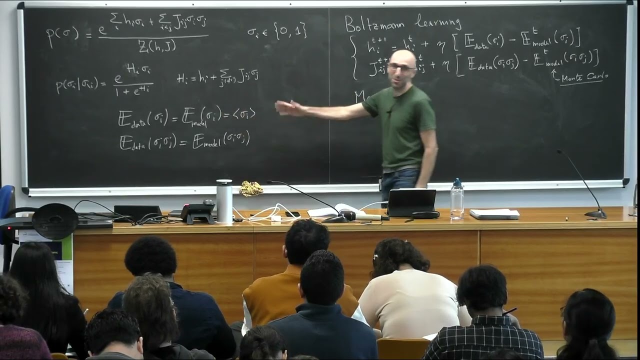
From Statistical Physics to Data-Driven modelling in Biology - session 8

Okay. Um I guess we can we can start. So um uh before I forget the the I prepared the exam. So the exam will be in the same format as the one of u the course of Maro Vastori and Bruno Luro. So it there will be 20 multiplechoice questions and you will have to uh answer uh without using notes or uh electronic devices. Okay. Of course. So I mean these are simple questions on the on what I said in the lectures and I think it I mean if you follow the lectures you should be okay. Okay. So now to conclude the the discussion I wanted to finish the discussion on graphical models and then show you an application to proteins. So let's start from the let's start by concluding the discussion on graphical models. So we are trying to infer a graphical model which means a model the probability distribution over our data uh which is made by local terms one per variable plus interactions and these interactions form a graph where the graph is u the set of pairs i j such that j is non zero. So there is a direct interaction between the two uh variables. Um we have seen in the case of gausian variables that we can compute many things explicitly and we can infer we we have an an estimator for the matrix of the uh couplings uh and we can regularize and we can study what happens how many data we need and so on and so forth. uh but okay in most applications you don't have gausian variables you you have more complicated uh things and in particular you you can have categorical variables so now we move to the case of categorical variables and for simplicity today let's for for this discussion let's restrict to binary variables so for example 01 or minus one1 if you prefer but here it's it's 01 So you can think to these binary variables for example as if you have recordings of neurons in a given bin time bin you can say zero means that the neuron is not spiking and one is the neuron is spiking and you would like to infer these parameters. The hi will tell you what is the probability of neuron I being active and the jig will tell you what is the coupling between neuron I and J which means which is related to the probability of being both active. Okay. So from this then you can infer uh you can get information about your your system for example which neurons are the most uh the strongest interacting and so on and so forth. Um so we we choose this model uh which is a Boltzman distribution of an easing model with local fields and two body interactions and we said we can motivate this choice in two ways. One we can say okay we want to do maximum likelihood inference. So we choose a likelihood. So in this case this will be our likelihood of the data sigma. Sigma are the data uh given the parameters H and J. I don't write it explicitly but this will be the the probability of sigma given the set of parameters H and J. And you can say okay I choose this likelihood because it's simple. It's the exponential of of a Hamiltonian with one and two body interactions. And you could if you want add free body interactions, four body interactions then you would have a more complicated graphical models and many more parameters. So to start with we stop at the simplest non-trivial term. Of course if we don't put this then we have independent variables and then uh we don't have information on interactions. So this is the simplest choice if you want of for the likelihood of of a graphical model. Or if you prefer you can say we want to do maximum entropy. And so this would correspond to the maximum entropy distribution with the constraint that the expectation of sigma i on the data is equal to the expectation of sigma i on the model and the same for sigma i sigma j. So this is also the maximum entropy distribution that is consistent with fixing the firing rate of each neuron and the joint firing rate of each pair of neurons if you think about neurons. Okay. Um I also told you yesterday that in these in these models you have an overparameterization if you write it in the most general way because in principle if you have two states here you should have a 2x2 matrix and here should have two fields but you can fix you can always remove one field on each side and one line and one column of the matrix. So if you have binary variables you can reduce to to this form with only one field and one coupling on each um pair. Okay. So now the problem is we have data how do we get the hi and the jig. So the first possibility we explore this boltzman learning. So Bzman learning is the exact way of getting the the the fields and the couplings in in this context is it is exact in the sense that um either if you do maximum likelihood or maximum entropy in both cases if you maximize the entropy or maximize the likelihood you obtain that both quantities are concave so they have a unique maximum. The maximum is obtained when the moment matching condition is met. So you have n field you have l fields and l * l minus one /2 couplings and here you have l equations and l * l -1 /2 equations. So these equations fix everything. But in order to solve them, you can just do gradient ascent on the likelihood or on the entropy as you want. And this will give you iteration equations of the form. If you if your model has too low uh firing rate for neuron I, you increase the field so that you increase the firing rate. So this will give in general something like um something like this. If your firing rate is too low, you increase the field. If it's too high, you decrease the field. And the same for the couplings. So this will converge to the unique maximum if you of course um if you have if you choose wisely your learning rate of course otherwise you can have convergence problems and okay here it's the of course it's the model at time t so you will have couplings and fields that evolve in time where time is the number of iterations of your algorithm And after a long enough time this will converge. The the problem with Bzman learning it is exact. So once you are at convergence you have your probability distribution and this is really the maximum entropy distribution. The problem you have a certain number of problems. First of all um okay first of all this is not the problem. This is an advantage. these two things you compute them at the beginning of the algorithm and and then uh and that's it. So this is particularly good when you have many data. If you have many data, computing these things takes a bit of time but you do it once and then you are done. You you have your uh L magnetizations and you have your L* L minus2 uh correlations and and you store them in memory and you run and and it's okay. So when you have many data this is an advantage but the problems are that you have to compute these two quantities and to compute these two quantities as you know you cannot compute magnetizations and correlations for uh an arbitrarily complicated easy model. So you have to do Monte Carlo. So you will need Monte Carlo sampling to compute these things. And here you have a disordered easing model. So you know that when you do Monte Carlo in a disordered system, you can have convergence problems of the Monte Carlo. So the Monte Carlo can be slow and this can take time and if you're not careful enough, you have bad estimates of your expectations in the model and the Bzman learning as convergence problem. So there is a long series of studies of how to properly do the training and there is a lot of progress in the last years in particular thanks to the work of the group of batteries sane. So they found various way to improve the u the strategies to do Monte Carlo in a proper way. So you can check their work. It's very interesting. Now the other problem is that also the the Bolzman learning itself even if in principle it's guaranteed to converge can have convergence problems in the sense that okay it's convex but still it's a high dimensional space and a convex function in a high dimensional space can still have very flat directions. So sometimes you can have also a bit of a slow convergence of the Bzma learning. So even if you have a good estimates of the mo of the moments of the model uh this can take some time and you have to be careful in the choice of the learning rate and so on and so forth. So overall this is a good strategy but okay in the modern implementation that we have it will require maybe one hour or few hours on a GPU to have a good convergence in a model with maybe 100 in a protein for example I will show you with 100 sides uh it will be something like that and then when you increase the size of your data it it it becomes slower and slower so you can have problems So this is why people have explored alternatives in particular in the in the past when computers were slower and uh there were also less data and so on. So there are there are other methods we have seen the mean field approximation. So the mean field approximation is based on applying minfield to the easy model. And when you do that uh what you get we discussed yesterday you get okay now let's call just to simplify let's call this the magnetizations let's call the average over the model in in this way. So the mfield field equations give you an equation for for the magnetization that has this form that is obtained as we discussed yesterday from the from the conditional probabilities. And so here the average of h is equal to h i plus the sum / j of uh jig j sigma j average. So from this equation you can take a derivative as we did yesterday and you obtain that jig j is simply c minus one i j for the off di minus c minus one for the off diagonal elements when i is different from j the diagonal elements of j we suppose they are zero we we we don't have a self interaction because there is already the field so Okay. Um, so from this you can say okay if I want to fix the moments I want cig to be equal to the cig of the data. So I will put here cig of the data and I get jig. And then if you want to get hi well you can obtain it from here. You assume that the sigma i the magnetizations are the ones of the data and so here you know the j you know the magnetizations from the data and you can you can solve these for the fields okay so this is a very simple uh procedure you don't have to do any Monte Carlo you just invert you get from the data the correlations and the magnetizations you invert the correlation matrix this gives you the coupling and then you from here you get the the fields Um so this is very efficient computationally. The problem of this the disadvantage is that if you uh then it depends on what you want to do. So we I will discuss it a bit more systematically later. But once you have this model you can do two kind of things mostly. One is to try to use the parameters to infer information. So for example from the J you get the direct coupling between two variables which is a good measure of their interaction. So if you want to do that the mean field is usually a good uh approximation. It gives you a good approximation for the couplings. But the other thing you might want to do once you have this is to generate new configurations of your system. So you might want to use this as a generative model which means I learn a probability distribution from the data and then I use my probability distribution to generate new data. For example, if you have proteins you maybe you want to generate artificial proteins. Um in that case mean field is usually not a good uh thing in the sense that when you go if you take the mean field parameters and you put them here and you sample new configurations of the sigma from the distribution what you see is that the new configurations that you are sampling are not uh very similar statistically to the training data. So typically the moment match for example if you look to the moments they are even if you infer from by matching the moments because you're doing an approximation the moments will be quite different and if you look at threepoint correlations they will be also different and so on and so forth. So mfield is good to get an idea of the parameters but it's not particularly good if you want to use it as a generative tool. Okay we will come back to this. So >> excuse me. >> Yes. So when we when we use midfield approximations, we don't need to do the learning. >> Mhm. Exactly. >> Actually find the solution of the problem >> in in in one shot. Basically you I give you the data. I will show you an example. I give you the data. You compute from the data these two these two quantities which is easy. You just do an average over the data of of these things. And then uh from this the cig is just uh cig is uh sigma i sigma j minus sigma i sigma j. So from if you if these are given by the data you you have your estimate of CI from the data and and then you have an L byl matrix that you have to invert. So inversion of an L by L matrix takes L cube or something like this. So you get you get this and then these are L equations that you solve. So it takes time that's that is a something like L cube. Here the problem is that the Monte Carlo can take a time much longer than L cube. So uh that that's the issue. >> But the point is that min approximation is not a good approximation always. Right. >> Exactly. So >> then we need to do both learning. >> Exactly. So it depends on what you want to do. Minfield approximation is in many applications it's a good appro approximation to get an order of magnitude of the couplings. So if you are just interested in knowing for example which are the strongest couplings then it's a good idea it's a good approximation but if you put if you but you make mistakes on the couplings. So if you put the couplings back here and you sample new configurations the mistakes you make will accumulate and the configurations that you sample will be quite different from the training ones. So you know if you want to generate if you want a good generative model what you want is that the you learn a probability distribution that is able by sampling to generate states that are similar to for example if you do image you start from images you learn a distribution then you use the distribution to generate new images and you want the images that you generate to be similar to the ones. So if you do mean field this is typically not the case. Okay, it's not a good generative model. Okay. So what what else can we do? Uh we can do s likelihood maximization. So I don't I don't have uh enough blackboard. So let me erase this. Uh so how does it work in this case? It's very easy. So you start from the pel likelihood. So what you want to learn when you do pel likelihood maximization is you directly want to learn from the data the conditional probabilities. Okay. So what you do as as we did for gausian uh uh uh as we did for gausian variables you define the likelihood which is 1 / m times the sum over your data of the logarithm of the probability sorry this is well okay this is of the probability of sigma i condition to the other variables. So here you have data. So on each data point you have the value of sigma and you have the value of all the others. So you compute this and you maximize the likelihood. So you will have one likelihood per variable and you can do it separately or you can sum them. It's the same. Why? because this thing is 1 / m. So when I take the logarithm of the of this I get um h i sigma i minus so and this will be minus the log of 1 + this. But you see that h i the the local field acting on variable i depends only on the field associated to the same variable and the couplings associated to that variable. So this quantity does not depend on all the fields and the couplings. This depends only on hi and the vector ji that contains the couplings of i with with the others. So this is one of the one row of the matrix jig j. So this means each each cellular likelihood associated to each variable you have l variables. So you can imagine that you have your string of L variables sigma 1 sigma 2 sigma L and you want to learn you want to learn the probability of sigma i condition to the others. So you you will have a local field HI and you will have couplings J I J and from each cell likelihood you learn one field and L minus one couplings and when you put them all together you will learn the whole thing but because each cell likelihood only depends on these two things it's the same to maximize each have the likelihood separately or take the sum you could take the sum over i and maximize all together it's it's exactly the same okay now what is the advantage here the advantage you see that you don't have the partition function here why because well here in order to normalize the joint probability of all the variables you have you have the partition function and the partition function is the sum over all the variables of the numerator so this is a sum over 2 to the L states. So it takes exponential time to compute and so you have to sample from Monte Carlo. But here if you fix L minus one variables when you normalize you only have two states for the variable sigma I so the sum over two states can be done and you get one plus this and so it's it's everything is is explicit and you don't have to to take this normalization. So this means that the the likelihood can be computed uh explicitly and this is the expression. So now when you take derivatives you can write explicitly the the derivatives. Okay maybe I will not do it but you have you have it in the book. So when you take the derivative with respect to hi for example here you have an hi so you will get something like 1 / m s m of sigma i m and here you have minus 1 / m s m here you have 1 / 1 + a. when you take the derivative you have something like this and this should be zero. So you see that the derivative of the likely well okay I'm doing it so let's do it let's do it just for the fields the derivative of the likelihood gives you a a sort of a moment matching condition which actually corresponds to the ken identity so this is telling you that the expectation over the data of sigma i should be equal to the expectation over the data of this is sigma IM sigma IM times the conditional probability of of sigma IM. Okay. So this is the same as the Ken identity I discussed yesterday but with the average over the model replaced by the average over the data. Anyways this is not very important. What is important is that you can compute this gradient from the data. So you can do gradient ascent on the likelihood. So at each step you will do something like dhi over dt equal to some learning rate. Let's say one over the learning rate times the hi the hi over dt is equal to the gradient. So you do gradient ascent and at each step you have couplings. you have H and J. So you can compute from the data this HI. The problem you see that this is very good if you have if you don't have too many data because if you have a lot of data then here at each iteration you don't have to do the Monte Carlo sampling because you can compute everything exactly from the data and you don't have noise. This is a deterministic equation once you once you have the data you see. So you you don't have to worry about sampling Monte Carlo and sampling noise and so on and so forth. But if you have many data at each iteration of the algorithms you have to compute these things from the data and so it can take time but this can be solved. You can do many batches on the data and things like that. So in general this will converge uh quite fast. Okay. Uh yes. >> How does the sigma appear in the second? >> Yes. because h I uh because there is this um oh well no you're right there is no sigma here uh this this is wrong sorry uh you're right thanks there is no sigma so the >> yeah it should be it should be yeah it should correspond to the col identities so let's check but yeah you no no it's it's correct it should be like is thanks. Yeah, I'm differentiating with respect to hi. So there is no sigma. No, no, it's it's correct. So this is the correct equation. Sorry. And and the colian identity has no sigma. So it's okay. Thank you. Okay. So um so the advantage of the so let's erase this um and also this. So the advantage of cellular likelihood is that it's computationally more efficient than BSA learning but again the disadvantage is that and and okay you get good estimates of the couplings and the fields much better than in field. The disadvantage is that again it's not easy to use it to generate new uh configurations. Why? Because okay first of all the problem is you remember you can show that if you have infinite data then so the likelihood maximization is the same as bzal learning and this is we showed it for gausian variables but it's true also for uh in this case so if you have infinite data this maximizing the like likelihood will give you the same as bzman learning but okay so in that in that case it's okay but If m is finite then the problem is that your matrix jig j has to be symmetric. Here you are inferring each row each row is is being inferred by different data. And so in general you will get a nonymmetric j because of noise of the finite sampling that you have. So first of all you don't know how to put it here because here the j are are symmetric by construction. If you have different because you see J is multiplying sigma sigma J. So if even if it's not symmetric because this is symmetric the anti-ymmetric part will disappear. So you you then you have to decide what to do. One thing you can do is to symmetriize by hand. So you can say okay for example I I put in the distribution the average of JIG and JI and then I try to I plug it here and I try to generate new data. So people tried and it's not very good. So once again because of the small mistakes you make on the J when you use it as a generative model you don't have a very good uh correspondence between what you generate and what was in the training set. The other thing that you can try is to to say I keep it I keep it as it is. So I I I forget about the joint probability. I know the conditional probabilities. So you can try to do to generate new data by saying okay I start from a sequence. I choose so I have sigma 1 sigma 2 sigma l. So I I start from a random uh sequence. I choose a site I and I say okay now I know the probability. I learned the probability of sigma condition to the rest. So I draw a new sigma from that probability. Okay. So now I choose another site and I draw this one from the conditional probability. So I use the set of conditional probabilities to uh sample new states like I would do in Gibbs sampling. I do it many times and I hope that I converge to something good. Well, we we tried that and it doesn't work. So typically the problem is that your conditional probabilities because they are learned from finite data are not exact. So you have you have mistakes and you have inconsistencies between them because the couplings are not symmetric. So they don't respect the the fact that they all come from they should all come from the same joint distribution. So you make mistakes when you do this sampling and that accumulate and then your thing goes your sampling goes to states that are that are not statistically similar to those that you have in the training set. So once again it's and okay I I'm not going to I mean if you're interested I can show you offline I can show you results but I'm not going to discuss this too much. But then so once again this is not a very good model for generate to to generate things and this is something that is also uh I think uh used in more like modern machine learning architectures like language models. So you see that cell the likelihood maximization maximization is very similar to what you do I mean for those who know language I think you all know language models. So it's very similar to what is called masked language modeling. So you have your string of text and what you do is to learn a model that will learn to predict a word based on the context of what is before and what is after. So again you try to learn the conditional probability of a word given the rest of the string and you train your model by randomly masking some sides and learning this conditional probabilities. So so the likelihood is very similar. So typically in this like modern architectures you have a string of text that is input in a deep network of like transformers and stuff. And so you start with your text that is here. You input this in layers of stuff. Okay? And then you so you input this. You do many things and you end up with logits at the end that give you the probability that are trained in such a way to give you the probability of one word in the context of the rest. Right? So this is what so the likelihood does here. Here it's a very simple architecture where you have your your data right you pass you can see that you can represent this as you have your data sigma 1 sigma L you apply a very simple linear layer because what you do here you produce the fields by doing a linear combination of the input plus a constant. So this is what a linear layer would do. So here you have if you want a linear layer that will take these as inputs. It will produce the HI here. So H1 HL and what you do is to train this HI are the logits that you train to reproduce what you have in the output. So you take the same configuration here sigma 1 sigma L and you learn this in such a way that H1 will give you the correct probability of sigma 1. Right? So it's it's it's a very similar idea except that this is a just one linear layer plus a soft max. If you want here you do a soft max. So s likelihood is like masked language modeling where you have a linear layer in the soft max and you have a also here you work with fixed size while in in language model you try to work with strings that can have a variable size. So you have all the problem of positional encoding and so on and so forth but the idea is similar. Okay. So also in language modeling what you know is that if you try to generate a text by taking a a starting text and you and predicting the the words at random uh based on what is before and what is after it doesn't really work. What people do when they want to generate new text is to use a different uh procedure which is called auto reggressive uh uh generation. So how does it work? It's it's basically a variant of this in which you say okay instead of using the conditional probabilities of each variable in the background of all the other variables I change my setting. So auto reggressive models. So in in autogressive models what you do is you you use the fact that uh the joint probability of L variables is always um can always be decomposed as a chain of joint uh of conditional probabilities. So you say okay my P of sigma is not this one now. So forget about this one. I will write it as P of sigma 1 P of sigma 2 condition to sigma 1 P of sigma 3 condition to sigma 2 sigma 1 up to P of sigma L condition to sigma L minus one sigma 1 okay this is exact you can always do it and now you say okay let's try to learn these things okay so I do maximum likelihood so my likelihood is going to be 1 / m sum of the log of p of sigma m where sigma m are my data and well because the this is a product you get you get a sum of likelihoods let's say l1 plus l2 plus l3 plus l where each likelihood is the lo the average of the log of one of these terms and now what you do is to make a model for this and try to learn the each term. Okay. So the simplest model is always the same. If you have this kind of variables you can say okay the probability of sigma i conditioned to what is before. Now it's not conditioned to everything but only to what is before. So now you're changing the architecture. The probability of sigma condition to what is before can be written as exponential of a field times sigma i divided 1 + exponential of the field. This is always the case for binary variables. And then I write the field in the same way. So I write this field as a local field hi plus the sum over j but now smaller than i not different before it was different from i of j i j sigma j. Okay. And then for each term I have a field. So I have h1 that h1 is just a field. H2 will be H2 capital H2 will be a field H2 plus J 21 sigma 1 and so on and so forth. So what you're saying is that again this is an auto reggressive architecture where each field is a a linear each field capital H is a linear combination of the input but the input is restricted only to the previous ones. So for example, H2 will depend only on sigma 1. So here you get an auto reggressive linear layer where H2 depends only on on sigma 1 and H3 depends only on sigma 1 and sigma 2. Sorry. So let's say H1 is a constant. H2 depends on sigma 1. H3 depends on sigma 1 and sigma 2 and so on and so forth. And the last one will depend on all the previous ones. Okay. When you train this by maximum likelihood, when you maximize the likelihood, you get you get equations that are very similar to the ones of the likelihood with the only difference that these sums are only on the previous ones. And you see that each of these likelihoods in this architecture depend I mean depend on different parameters. So the first one depends on on uh um small H1 L2 depends on small H2 and J12 sorry J21 L3 will depend on H3 and J31 and J32 and so on. So each term can be maximized separately. So basically you are learning separately a model that gives you the probability of a spin condition to what is before. The number of parameters however is the same. Uh I mean in the thing is if you do boltsman learning you have okay you always have L fields and then how many couplings you have if you do boltsman learning the couplings are symmetric. So you have L * L - 1 /2 and also mean field. If you do the likelihood the couplings are not symmetric. So you have L * L minus one. So you have twice the number of couplings. But this is not really consistent. So you should symmetriize them or should do something. Um and if you do auto reggressive you still have L * L - 1 /2. Basically your matrix is lower triangular instead of symmetric. You say that there is zero couplings with the future and there is a coupling with with the past. Okay. The the good advantage of the auto reggressive models is that they are generative because once you have these parameters you have a consistent way of generating a new configuration which is just you generate the first spin then you generate the second spin condition to the first and so on and so forth. So now maybe what I can do is it clear the architecture I can try to do some table I don't know if you want to compare the different methods so let's say you have bolts learning you have mfield you have s likelihood maximization and you have autogressive models and well you can you can ask a few things. You can ask many things but for example you can you can ask the computational uh efficiency and well mean field is very fast. you just have to invert the matrix. These two have similar computational efficiency but and it depends a bit of on how many data you have. If you have many data can be a bit slow but then you can use batches. So this is good let's say a bit slower than than mfield and bzman learning instead is quite slower than the other methods. Okay, still doable if you have a GPU and if you have I mean also on a GPU actually but it takes a few days. Uh and you I mean it's it's a bit slower then you can ask what kind of information you you can get from the couplings and the fields and this is I would say comparable for these three methods. So if you for example try to look at the biggest couplings that you have uh we will see in proteins that the biggest couplings are related to contacts you have good prediction of contacts from from all of these methods. Um so the likelihood maximization is a bit better than in field. You can okay you can discuss but they are all good from the auto reggressive it's a bit more complicated to interpret the couplings because in this in these three schemes you are really inferring a graphical model even if this is exact and this is approximate okay in auto reggressive in the auto reggressive case it's a bit different in the sense that you're not inferring this model so it's not the jig are not really the the couplings you are inferring this chain of joint probabilities. And so if you want to get the coupling strength of two variables, it's a bit complicated because what you should do is for example, you should take the log of the probability call it uh energy somehow or Amonian. But this this will be a sum of all these terms. And you can see that effectively you have many body interactions because you have I mean even if each of these terms is written as a as a as a the exponential of two body interactions in reality in the denominator there is the field that depends on all the others and you can see that you this will induce many body interactions. I maybe I will not go into the details but so if you want to get couplings what you have to do is to start from a sigma from one state and make change two spins and see what is the variation of energy when you change two spins and so you can extract the coupling from there but the couplings will depend on the rest of the spins because you have all these. So you can get effective couplings and they carry similar information if you do that but okay you have to be a bit careful. So let's say uh you have to be careful. Okay, this is not a graphical model in the same sense as this. So you have to decide then what you do w with your model. >> So so you're saying that we have to fix or take the the copings pair to pair fixing the others and see what is the effect on the energy. >> Yes, this is one way of doing it. So you take a reference state you make two you change two spins for example you start from old zero you switch I and J to one the difference in energy should be if you want to interpret this as aonian of this form when you do when you switch on two spins the difference is the energy will be jig plus hi plus hj so you will then you remove h i hj and and you get jig so you can infer coupling. The problem is that the coupling that you get depends on the state of all the other spins because you can see that the this denominators that you have here contain effectively many body interactions. So you have to be careful. >> Yes. that um will have the same performance or similar performance if we take like random states initial states. >> You mean to estimate the coupling? >> Yes. >> Yeah. You I don't know. It really depends on the problem you have. That's why I'm saying we tried on proteins and on proteins it works in the sense that the couplings don't depend too much on the initial state. So you can take one reference you can average over some initial states but then if you have another problem it could be so just I'm I'm just saying be careful that this this the hi and jig that you get are not the one of the graphical model they are different so you have to decide what to do them and sorry maybe here we can say this is training computational efficiency then the other thing is that now you can once you have these models you can say let's try to generate configurations. So if I generate new states, these ones will work. These are consistent probabilities that will give you good states. So for example, if you generate many states and you look at averages of observables, they will be the same on the generated states and on the training set. These typically do not work. Okay, they are not good at generating new states. And on top of that, you can ask what is the computational cost to generate a new state. And here it's it's slow because if you want to generate a new state from the Boltzman distribution, you have to do it by Monte Carlo. So it can be slow. So the good thing of of auto reggressive models is that it's it's very fast because you can generate in this sequential way. So you start from a sigma one then you go on and at each step in order to compute the conditional probability you have to you have to compute this local field that takes order L operations. So in the worst case it takes order L square operations to generate a new state while in the Monte Carlo it could be even exponential in L if you have a I if your system has metastable states and so on and well for these two I don't say it because I mean it's the same as Bzma learning but it's not even good so you don't want to do that. So okay so depending on what you want to do you can choose your uh your right uh the best approach. Um there is one last thing which is and I will show you an example of that as well which is the dynamics. So you you might be interested not in generating states in equilibrium from this probability distribution. You might be interested and I will show you why in starting from a state and generating a dynamical uh process that starts from that state for example by proposing mutations and accepting them with this probability or this probability. So in that case it's much faster to do it with Bzman um machines than without a regressive model. Because auto reggressive models are very good if you want to generate a new configuration from scratch because you say okay I I don't have a configuration so I I generate sigma 1 then then sigma 2 then sigma three then sigma l and it's it's very fast but if you want to propose a mutation and and accept it with this probability then it's it's very complicated because if you have a state and you want to change sigma one sigma in the middle you have to recomp compute ute all the probabilities of the following spins. So it takes a lot of time. Okay. So if you want to do one mutation of of your configuration with this, it's very slow. While with this, you know that if you want to do Monte Carlo and you do a single spin flip, you just have to compute the energy change and you do metropolis and it's very fast. So really depending on what you want to do, each of these architecture has advantages and disadvantages. So these are complimementaryary approaches and you can choose your your favorite one. Okay. So there is one last thing I would like to say. Um yes >> um can you explain again the difference between >> yes so um you can say so when you want to generate a new configuration you would like to generate one independent sample from P okay so you don't have any previous information you say you have a probability you want to sample one configuration from this probability here It's very easy because I draw sigma one. I have two states. I I know the probability. I draw one. So I know that my first spin is one for example. Then I know the probability of sigma 2 condition to the first. So I draw sigma 2 and again it takes you have to do one operation. You you have to do to compute the field and then you have to do one operation. computing the field I erased it but the field is a linear combination of so it's of order L so at each step you it takes of order L operations to compute the field and one operation to draw the new state so you have L states each each one takes L steps so you have L square operations and you get a new configuration here instead you don't know how to sample from this distribution because the partition function is uh because they are all correlated. No, the spins are all correlated. So you don't know how to start with one because you should compute the marginal. But to compute the marginal, you have to sum over two to the L states. So what you do is you do Monte Carlo. You start with a random state. You propose a flip. You accept with the metropolis step and you do it many times until it converges to equilibrium. The problem is that it could take exponential time to converge to equilibrium in L if your system is disordered and metastable and so on. Okay, this is okay if you have experience with Monte Carlo this will uh talk to you otherwise not really but it it's you have to try and and see. So it will take a lot of time. So this is what why I'm saying generating from scratch one equilibrium configuration is low for ballsman learning and is fast for auto reggressive models. I mean can be slow then it depends on the problem but instead if you already have a state and you want to know and you want to propose mutations to that state for example I will show you in proteins this can be a way to model evolution so I start from a protein I know and I want to propose mutations so then I want to know I I have a state I change one spin how does the probability change okay here it's easy because the partition function is the is fixed is a constant. So if I want to know the variation of the probability, this depends only on the numerator. And if I change one spin, I have to change L terms here. So it takes order L time to compute the change in in probability and then I can accept or not with Metropolis weight. Here it's is lower because if you change one spin for example if if you change sigma 2 this will affect this term but it will also affect all the following terms. Okay. So you have to compute the if to compute the variation of P when you do one mutation you have to do you have to compute the variation of all these it's not much I mean it's a factor L slower basically than than Monte Carlo but so if you if L is 100 you lose a factor 100 in your in the time it takes to to propose a mutation to sorry not to propose to check the effect of a mutation okay >> so in the dynamics you want to check the energy variation between >> exactly Exactly. So the energy is the logarithm of the probability. So in order to check the variation of energy, you have to check the variation of the probability. Here it's very easy because the log of the probability is just this plus a constant that will not change. >> So the first case is you just need one step, right? >> Well, L steps because if you change one spin, you have to compute the effect of the change of all the other. You have each spin is coupled in principle to L spins. So it takes L operations in Boltzman distributions here it takes L square operations because you have L terms and each of them is a sum of L things. So okay anyways this is uh just to give you an idea. Now um the last thing I want to discuss and then we go to the protein uh application is regularization and maybe let's just do very quickly. So you can do up to this moment I didn't I didn't put any regularization. So in principle I am inferring a model with L square couplings. I might want to maybe I I I might suspect that my coupling matrix is sparse. For example, if you want to infer I don't know a two dimensionalizing model then your couplings are non zero only if you have nearest neighbors. So many couplings are actually zero. So you might want to enforce that. So there are many ways you can add an L1 regularization to the to the likelihood. So when you do for example in Bzman learning when you do your gradient ascent you can add an L1 norm and you can uh regularize that way. Um there is also something we did uh over the past years that I want to just very quickly explain that is works quite well which is to activate the couplings one by one or start from a fully connected model and remove the couplings one by one. So how do you do that? So for example, if you activate the couplings, the idea is very simple. So you start from a model with zero couplings. So you start with J equal to zero. And if you start with J equal to zero, you only have the fields and you can learn the fields very quickly by as I discussed yesterday. So if you don't have coverings, the fields are just the logarithm of the frequencies. uh normalized. So you you have the fields at the beginning and then you can ask okay if I add a coupling what is the the variation of the likelihood okay so if I say my my Hamiltonian here is equal to minus sum / i of h i sigma i minus sum over i j of j j sigma i sigma j and in such a way that this is e to the minus h over z okay the minus sign is the convention of physics now okay so let's say I start from some h0 for example h0 might be the one without any coupling and I add the coupling. So I say sorry I say H is H0 minus I add one coupling I J. Okay. And the question is how does the likelihood change? So the likelihood the variation of the likelihood is 1 / m sum over m of the logarithm of p minus the logarithm of p 0 right where where p is the exponential of minus h / z and p 0 is the exponential of minus h0 / z 0. So what is this? This is 1 - m times the sum / m of minus h of sigma m plus h0 of sigma m uh minus log z plus log z. Okay. Now the difference H0 minus H is simply JIG sigma I sigma J right. So the first term is Jig J times the average over the data of sigma sigma J which is something I I have And this term is plus um well we can write it as minus the logarithm of zed over zero where zed and zero are constants. So when you do the average over the data they remain constants. Okay, this seems difficult to compute because it's a ratio of partition functions. But actually, if you look at what it is, Z / Z 0, you can write it as the sum over the sigma of E to the minus H divided by sum over sigma of E to the minus H0. But H is H0 plus Jig J sigma I sigma J. So this can be written this is the partition function of h0 and this is if you factoriize the exponential this is the average over the average of jig j sigma i sigma j over the model h0. Okay. So now the average of this is actually very easy to compute because can I I will erase this okay to make some space because jig j is either zero or one. So this is e to the jig j if sigma i sigma j is equal to 1. This is uh e e to the jig j times the probability that sigma sigma j is equal to one which is basically the expectation of sigma i sigma j over h0 plus if sigma i sigma j is equal to zero this is one and the probability that sigma sigma j is equal to zero is one minus this Okay. So this thing in the end is given by jig figj where figj is the frequency of sigma i sigma j being both one in the data minus the log of e to the j i j p 0 j where p 0 j is the probability in the model of sigma i sigma j being both active plus 1 minus p zero. So if you're doing Bzman learning, you know during the Bzman learning you have to compute you know the frequencies of the data. This you compute at the beginning but you also know the probabilities of your model because you are doing bolts learning. So the idea is you start with without couplings you do bolts learning and from time to time you look at your couplings and for each pair I j you compute the variation of likelihood that you would have if you activate that coupling. So you have it and so you can maximize this over jig to find the best possible value of jig and you can compare all the possible j and you can choose to activate the couplings that maximize the likelihood. So you can say okay at the beginning I have no couplings. I look at this I decide um I don't know 10 couplings that are the best ones. I act I switch them on and then I do my bolts learning only with those couplings. The other are kept fixed to zero. I converge and then I look again and I activate 10 more and so on and so forth. Okay? Until you like the result. What does it mean you like the result? You can what we did I mean this was our choice but uh um you can find a better choice if you want but what we did was to you can do two things. One is to check the usually we check the Pearson correlation between the correlations of the model and the correlations of the data. So you have L square over two correlations. You can do a Pearson correlation of this. So you do this and so usually we check this and when it reaches something like 95% we consider the model to be good. This is just based on our experience. And what you see essentially as a fraction as a function of the number of couplings that you have let's say if you look as a function of the how can I call it now uh well okay number of couplings fraction of couplings that you have activated this usually does you plot if you plot this quantity as a function of the fraction of couplings that that this means This is without couplings and this is with all the couplings present. This usually you get something like this. Okay. And this is about 95%. I mean 95% is what you typically get from the best model because you always have a bit of noise. So you can say okay maybe I I stop when I when I reach 95%. Um but there is something else you can do which is to look at the entropy of your model as a function of um of the number the fraction of couplings and what you what we see is that actually the entropy has a maximum at some point and then it goes down. Why? Because if you have too few couplings, you in order to describe your data, you have to make them very strong. And so in the end, you lose entropy and uh well, if you have too many couplings, you are overfitting the noise and you are um and you are um so and you are again reducing the entropy. So one possibility to select the best model is to look to the mod to the to a model that is sparse and that's the fraction of couplings that gives you the maximum of of the entropy. And now I think this is this starts to decline a bit after the peak. So the peak is in the region where you already saturated to the good performance. So by looking at the entropy you can find the model that is fitting well the data and maximizing the entropy and so you can you can hope that you're not overfitting the noise. Okay. So this I think this is a at least for this kind of models this is a good way to regularize that you can do online during the the the Bzma learning. So you we we have a package that does this that is public and you can uh play with it. The other so you can do it either starting from zero and activating the couplings one by one until you reach the peak or you can do it starting from the model with all the couplings. You do the boltsman learning you converge and then you start removing the couplings one by one and it's very similar. You can check which which couplings are the ones that are that are um the most irrelevant by a similar calculation and you remove those that are irrelevant until you see that the entropy goes up and then you see that at some point the performance will go down and then you can decide where you stop. Okay. >> Yes. >> What is the role of the the variation of the line here to accept when you activate or when you decimate >> the difference of the >> Yes. Uh we use it to select which couplings to activate. We activate the couplings that maximize the variation of the likelihood. >> Okay. So we just like accept the activation of that coupling in the >> well you could do it in in that way but we do it in one shot. So we do the boltsman learning we saturate with a given choice of couplings and then we say okay we look at all the couplings that are zero we compute this for all of them and we sort them and we take the I don't know the top 10 or 100 it depends on this is this is a parameter in your learning you take the top n couplings and you switch them on and then you keep doing boltsman learning for a while until you converge and you do it again and the point is that estimating the change of likelihood is very easy because from the B during the Bzma learning you already have all the ingredients you need so you can do it without cost basically okay what did you do that you're getting >> uh I'm just this is true only for binary variables but you can generalize to multi-ate but if they are binary sigma sigma j is either zero or one it is zero it is one with probability given by this so with probability because this is the expectation value of sigma sigma j sigma sigma j is either one or zero. So the expectation value of a binary variable is is the probability of the variable being one. So with probability given by this this is one and so this is exponential of J and with probability one minus this this is zero and so this is one that's it and if they are multi-state you can generalize this thing >> what was again >> row is the person okay yes sorry I was fast on this so when you do when you train these models then what you can do is you take the CI of the data and the CIG of the model and you do a scatter plot and typically you have something like uh this with points. So you have L square points for each pair. You can compute the correlation of the data and the correlation of the model and you have a cloud of points and you can do a Pearson correlation of this to to understand how correlated they are. So one would be perfect correlation, zero is no correlation. So if you have zero it means your data like this and if you have one it's a perfect uh correlation. >> So row >> yes it's an actually between minus one and one it's a person correlation. So if they are like this it can be minus one but hopefully it's not the case. So you typically start from zero and you go up to something close to one when you train the model. >> Sure. Yeah. >> Here you just turning on one coupling or you're summing over and J. >> No, it's one coupling. just one. >> So for each coupling you can ask what is the change in likelihood if I turn on that one and then you can take the top uh n >> no okay um now we I can introduce okay I think I'm done with the theory and now I can introduce uh the application of these ideas to proteins. I mean of course you can apply these ideas to many data and in particular I told you the data of the neural recording of uh animals can be used in this way. This was done uh by many people but in particular first by the group of Bill Balik then more recently by Remy Monoson and Simon Aoko and then many others who is a Ferrari. Well I mean I can make a list of people working on this from the neural point of view. Um but I will discuss now the application to protein sequences and also can it can be done also with a DNA or RNA sequences. So uh let's see. Okay. So now I will use slides because I want to show you figures. So, these lights were prepared for a summer school uh last year and Oh, what's going on? Oh, no. This is not what I want. Okay. Okay. So, uh so, okay. Now, I I want to explain how you uh use these ideas uh in in biology. So in particular in protein um to analyze protein sequences. So what is the goal? Um so as you know uh well in I mean proteins are chains of amino acids polymers made of monomers that are the amino acids. So you can represent the protein by a string of letters. Uh and the letters represent the 20 possible amino acids. um uh so and and this in principle this encodes all the properties of your protein. So the proteins are produced uh as a linear chain that will then fold uh into some complex three-dimensional structure and this is due to the interactions between the amino acids. So they will fold they first produce what is called secondary structure of alyses and loops and so on and then this structure will fold into a 3D structure. Um once the protein is produced and folds then it will perform some function. For example you can imagine that I we will see some proteins that are used by bacteria to resist to antibiotics. So the protein will be uh transported to the membrane and then when the antibiotics arrive the protein will bind to them and cut them and degrade them. Okay. So this is what is called the function. So the idea in biology is that you have a mapping from sequence to structure to function. Um and what you would really like to know is uh given a sequence what is the function of the associated protein. The problem is that well the mapping from sequence to structure is somehow a mathematically well- definfined problem because you start from a string of letters and you want to map that into a physical protein which is a collection of uh coordinates of atoms. So both things are mathematically well defined and you have many data. So we have now I mean this keeps growing but we have a third order of 10 to the eight se protein sequences that are available in databases and we have of the order of 10 to the five structures. So the problem of mapping sequence to structure is quite well defined both from the point of view of mathematics and of data science if you want and I mean thanks to that it was solved as you know by essentially solved by alpha fold I mean it's not there are still many problems I mean in some cases it doesn't work but anyway now you can have reliable predictions of structure based on the sequence using these deep architectures And uh of course there was a Nobel Prize for it. So the problem is that the mapping from structure to function is much more tricky for several reasons. First of all because function is not really a mathematically well defined thing because it depends on many variables. It depends on the environment. So if you have a protein and you put it in a certain bacteria uh it depends if the bacteria can express it can transport it to the membrane uh then it depends on the chemical conditions whether it binds or not. So it depends on a lot of variables that can affect the result in a pretty uncontrolled way. uh so I mean when you talk about function it's really hard to define it properly what what you mean um but even in the simplest case so you can say okay now I do a well controlled experiment I have one species of bacteria I put uh my protein in there I have controlled chemical conditions I put a certain antibiotics in a given dose and so on and so forth so everything is well defined still measuring function is hard. So you have to do experiments where you grow these bacteria in very controlled conditions, you u put antibiotics, you select uh you have to define a growth rate and so on and so forth. At the end you come up with with a number. So for a given protein you can have a number for example the growth rate of a certain bacteria in certain conditions uh and and uh and that's a number. Okay. So you can get the number but getting this number is very expensive. So typically these are costly experiment both in terms of time it takes and money it takes. So you don't we don't have many data. We have experiments where people are measuring functions of some proteins in some conditions and there are more and more such experiments but still we are in a very very compared to the structures that are available we are in a very scarse data regime. Okay, we have few data and there will be more and more data but not so many data and again the nature of the data is subject to interpretation because you have to when you compare different experiments you have many things that are different and it's not like structure than structure is structured and kind of I mean there are proteins that that can have multiple structures but it's still a very much better defined thing. So this is to say that the mapping of sequence to function is a still a very open and unsolved problem and well you can either decide to do it in steps. So you can say okay I solve the structure and then I can try to map structure to function and there are people who work on that but what we will what we are doing is to try to kind of skip structure and go directly from sequence to function by using u this kind of models I discussed before why because you can include structure but it's still quite computationally expensive to include structure in in the game I will maybe discuss later why and so uh I mean uh we try to do things in the simplest possible way and given that you have few data and we try to start from the simplest things. So what I will try to do is to show you ways to predict function starting from sequence using these simple models and the few data we we have. So why we want to do that? Well, because if you learn something about the sequence to function relationship, then you can do many things. You can, for example, design artificial proteins that have certain functions you you might want to have. You can try to understand evolution. So try to understand how nature evolved certain functions and this means you have to understand also the impact of fluctuating environment, fogyny and all the process that go on in natural evolution. uh you might want to make models to understand what happens in the lab when you do an evolution experiment in the lab and these are more and more u being done. So you try to take a protein and you try to evolve it to develop a certain function for example or to differentiate and explore the space of uh sequences compatible with that function. So we try to do models to do that. And then you would maybe want to optimize protocols. For example, if you want to um if you want to design a library of uh sequences that have certain properties, is it better to do it with constant selection or maybe alternating cycles of low selection and strong selections, things like that. And the other thing is that we would like and people are doing it to generate uh mutational paths that connect different proteins and try to see for example how they can switch from one function to the other how easy it is to switch and things like that. Okay. So we try to I mean together I I work on this together with Martin Vite mostly and uh many other collaborators. We have a web page but there are many people of course that are working on this kind of things. So when I when I mean we I mean the the community of course uh well this is already done the advertisement of the book you have the book. Um so okay what are the kind of maybe I will I will discuss the kind of data we we can use and then we stop and uh tomorrow we uh we will u um continue the discussion. So the kind of data we have are natural data. So you have these databases where you can download proteins that have been sequenced sequenced. People sequence proteins for all kind of reasons. So typically they put them in these databases and and you can get the sequences and and what you I mean these databases are organized in families. So you typically have families of sequences that have typically the same structure and similar function. Okay. So for example, this is this betalacttoase protein that is used by bacteria to resist antibiotics. So you can get an alignment of sequences that are all uh folding into the same structure and they are doing something similar. So resistant to antibiotics. If you look at this, so you can align these sequences. I will not enter into the problem of sequence alignment which is a domain in itself but you can align them with standard methods. So when you align them you have to introduce sometimes gaps because during evolution maybe one amino acid can be removed. So you can have a gap here because here there is one more symbol. And so you have 21 now symbols in your strings that are the 20 amino acids plus the gap. And um if you typically look at at one family you have something between 100 and 10 to the five sequences. So between 100 and 100,000. And the the striking thing is that they are very different. So if you look to the if you take two sequences at random from the alignment uh they typically differ by 70 80%. Okay. So if you look at the number of mutations how many amino acids are different between the two most of the sequences is different. So so this means that there is a lot of variability. So nature found many ways of generating the same five and the idea is to say to use this as our data to train a model and we will train the model by maximum likelihood. So the idea will be that the model will give high probability to the natural sequences with the idea in mind that these are sequences that work. So we will we want to give high probability to the to the things that work. Uh in statistical physics language energy is minus log probability. So high probability means low energy. So the idea is we we try to learn our model in such a way that the natural sequences will have low low energy. And then we have other kind of data. So there are experiments where people take one protein and they do all possible single mutations of that protein. So on each site now you have 100 sites for example on each site you put all the 20 uh 19 amino acids that that are not in your reference. So you have 19 times 100 uh measurements of single mutations. Okay. And you can measure in these experiments these are called deep mutational scans. You can measure in these experiments the fitness which where fitness again is a measure of function and again it's not very well defined. So you you have to interpret the data carefully but it's typically the growth rate of some bacteria that have this sequence inside in some conditions. So you have a number for each sequence and this is supposed to give you a me an idea of the impact of one point mutation on a certain sequence. So from the point of view of the space of sequences, what you're doing here is taking one natural sequence doing all possible mutations. So you're moving very locally around it and measuring the fitness. So we can use this data in various uh ways. Then there are what is what are what are called invit revolution experiments. So in vit revolution works in this way. You start from a sequence for example one betalacttoase you take the the sequence and you you take the DNA you do PCR so you amplify the DNA but with a polymerase that makes mistakes. So you amplify the DNA but you introduce mutations typically one or two mutations. So you get the library of mutants that have one or two mutations. Now you take this DNA, you put it in plasmids, you put the plasmids in bacteria, you put the bacteria in culture with antibiotics and you see which ones survive. So now you have mutants that have survived. So they are good and you take out the DNA and you do it again and you keep doing it until you run out of money or time. And so in in these experiments typically they can follow and this is done in very controlled conditions. So you know exactly how much antibiotics you're putting and everything. And so you have an evolution experiment. The problem is that it's very slow. It takes a lot of time. So you can do in these experiments they did about 20 generations. There are more recent experiments that can reach 100 generations and even more recent experiments where they found ways to do this without having to take out and put back the DNA at each step. So they can do it online. And so they can reach 500 generations and maybe in the next years we we will be able to reach 1,000 or 10,000 generations. We can dream that we will have better and better data. So these are experiments where you start from a wild type a natural sequence and you look at how it diversifies in very controlled conditions. You typically reach a sequence divergence that is much smaller than nature because the time scales are very short. So you typically can mutate 10 20% of the protein but you sequencing is not very expensive. So you can sequence a lot and you can have many many sequences at the end of the experiment that you can read. The the last kind of data and then I stop is data where people choose two natural sequences that are at a certain distance a certain number of mutations and then they look at paths between them. So for example in this experiment from a few years ago they had two proteins that are one is fluorescent in the blue and the other is fluorescent in the red and they defer by 13 mutations and they did all the possible intermediates. So they you have two to the 13 intermediates where you take the two proteins and you mutate each possible site. And so they tested the fluoresence of all of the two to the 13 intermediates and they found this bottleneck shape where you have blue proteins here, red here and then in between you have a switch of fluoresence. So you can look at the space connecting two proteins and you can do similar things by reconstructing ancestral states. So you take two proteins, you reconstruct an ancestor and then you test sequences along the path that connects you to the ancestor. And so there are more and more experiments that also give you paths connecting uh different points. So the idea is to try to use this data or to model this data by what I said um up to this point. Um so that's the that's the goal. Okay. So next uh tomorrow to conclude the discussion we will try to make sense of this data using uh the kind of models I introduced. >> Okay. Thank you. Thank you Franchesco. So this evening we have this uh J start