Family Finance Surveys User Conference 2026 - Session 4

Hello everyone. Um it's time to start the last session of the day. So we have session four, new approaches to measuring living standards and household costs. And this session is going to be chaired by um James Smith, chief economist for the resolution foundation. So I'll just give everyone a moment to take their seats and then we'll pass over to James. >> I I see those stragglers at the back. Let's let's take seats. Uh you know who you are. Um I'm conscious this is the the final session. So I'm uh in between you guys and getting back out to some searing heat. So um I'm sure you're all desperate to do that. I'm James Smith. I'm uh chief economists at the Resolution Foundation. Uh for those that didn't hear that two seconds ago. Uh super interested in this session. I think you know the I'm afraid I haven't been able to join you for the full conference but um uh really looking forward to to having this discussion about measuring living standards. Uh so we're going to do the presentations one by one and then we'll come back and do a Q&A uh and I'll chair that. So I'm going to kick it over to Luke. You're going to speak at the the lect turn. You've got uh just under 15 minutes. We're running a tight ship here. So uh uh you're on the clock. >> Okay. Hello. Can you hear me everyone? All right. Yeah. Last session. So we'll get straight to I'm Luke Michael. I work at the Office for National Statistics. Um been there about 10 years working in a load of areas and I now currently going to be talking about the household cost indices. Um as you can see I'm in a suit. I didn't really look at the weather forecast. And of course I've I've not done too many inerson conferences. I'm used to them in online, so I don't know what I'll wear. So, suits great. It came in too hot. Um, but out of defiance, I'm going to keep it on until we finish. Um, right. Okay. Just before I begin my talk, has anybody heard of the household cost indices? And I'm really surprised because I didn't expect so many people. Great. Um, so that's what I'll be talking about today in the context of our consumer price inflation um statistics. So, for those that maybe don't know about the HIS or inflation specifically, here's a definition. Um, there's many definitions of inflation, but we stuck to the good old resource of Wikipedia, which feels incredibly old now. Um, so inflation is a general increase of the prices of goods and services in an economy. So, this is by far what the definition is. Um but high inflation essentially means that consumers can buy fewer goods and services or save less and the real value of household incomes and savings fall. So a good example is mobile phone bills as an example of a consumer contract. Um because money received from contractual payments don't cover the cost the same extent. Um for example with the contracts uh business from a business perspective they get less back as the cost increases. Right. So before I actually go into the household cost indices, you might be familiar with the consumer price indices index um which is the monthly bulletin. You've probably seen the news and the one that everyone's um worrying about when it goes too high, the one that went into double digits um after COVID. Um but you may not know there's a number of different elements and I think it helps to contextualize what HCI's are. So the CPI I'll start with which is it measures the average change in prices of goods and services purchased by households over time and it's the main measure of inflation in the UK used by governments and bank and the Bank of England. Um notably here it excludes stuff such as the um housing costs like mortgage payments and it follows international standards so it's comparable. Um we then have the CPI the casino prices own plus owner occupied housing. It's a bit like their CPI, but it includes um includes items that are specific to well includes owner occupying housing costs, which are costs associated with owning maintaining a house. Um and then I'm going to skip over HCI because I go into more detail about it since this presentation is all about it. Um and then we have the RPI which is we call it here a legacy measure um quite you it lost its accreditation um quite a few years ago and is discouraged by the ONS and will be no longer the same after 2030. Um, so they're the main ones and then HCIs. Before I kind of get into that, why why HCIS? So I've got a bit of a timeline here and it's, as you can see, fairly new, which is why I was so surprised about how many people did put their hand up. Um, so it was recommended originally by the Royal Statistical Society. Um, so that we have an inflation measure that essentially reflects household experiences rather than a macro economic or the whole economy. um work began in 20 uh 16 and it was called the index of house payments or the IHP before shifting that name to be the household cost indices. Um in 2017 estimates were a key milestone. It introduced democratic waiting which is what I'll explain a bit more what that means in a bit and a payments based approach and then subsequent years focused on expanding the coverage for example introducing housing loans insurance and student loans to name a few um ESCO price uh the ESCO group um then further expanding on the definition and in 2023 December 2023 we published our regular quarterly the publication of which I've been leading uh for the last two years or so. Right now it's the part I guess we all been waiting for. It's about the house of CS. So what what is it and why is it kind of different to CPI CPI and RPI? So it complements the CPI CPH to measure inflation across the UK economy as a whole. But the HCIs are designed to measure inflation. the inflationary experience of different household groups including income decels um tenure types retirement statement uh status and households with or without children. Um so the first important concept on here is the weight um the important differences. So the HCI's use democratic weights which means that the weights are based on an average household's share of expenditure rather than the total expenditure across all households which the CPI and CPIH use. So essentially they use different weights. I'll talk a bit more about weights in a further slide. Um basically in simple terms each household uses an equal uh has an equal influence in the calculation which means that it measures the measure is better suited um to understand the experience of the typical household. We also have a measurement basis. So the HCIs are closer to the payments based measure. So they aim to capture the change in payments households make for goods and services um rather than only measuring prices at the point of goods and services are required um contra in contrast to um the CPH. So this matters most for areas where timing of payments and consumption can differ such as in housing, interest or debt, um stuff like student loans. Uh and then we have finally owner occupied housing which you may go oh own owner occupied housing is part of the CPIH as well but specifically for this um it's the CPIH measures owner occupied housing costs using rental what we call rental equival equivalents which estimates what a owner occupier would pay to rent the equivalent property. The HCIs take a different approach to this and they capture the actual housing related payments made by the household such as mortgage interest, stamp duty, repairs and maintenance, dwelling insurance, group rent and transaction costs. So here is I guess a very quick overview of what I kind of explained to compare the two CPI HCPI versus HCIs. Um the main thing to take away here is that the HCI's CPH and CPI they're not there to replace each other. They are designed for very different purposes. Um which will be important some of the discussions. Um I wanted to focus a little bit quickly on the weights because and why they're important because it's one of the key and a key component between the HS and CPI. Um so inflation measures combined price changes using expenditure data and essentially weights tell us how important each item is in a basket. So if p pattern spending patterns change the weights need updating. So the index continues to reflect the actual household experience. This matters for the HCIs particularly because the weights are calculated separately from different household groups such as income decels and tenure groups. Um and plutoaucratic weights which are what CPI use reflect the expenditure shares of high spending households. So they are slightly different and weights are really important. The survey data allows us to reflect the average households and expenditure shares. Now, um we we've heard a bit about the living costs, well quite a lot about the living costs and food survey. Um and this is just a quick overview of how we use the living cost and food survey and national counts totals in the HCIs. 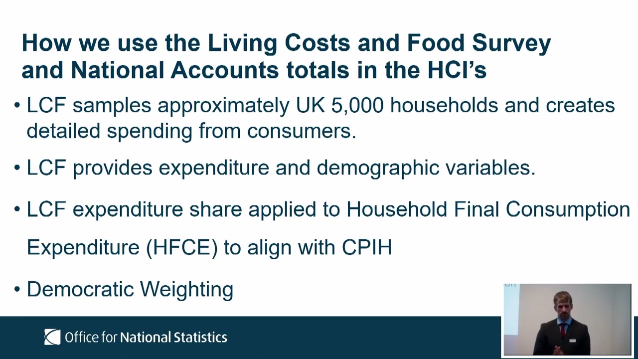Um so yeah the LCF samples as we've seen about 5,000 households and creates detailed spending from customers. Um so having seen how the expenditure weights are constructed for all household population the same framework is then extended to the subgroups. So most of the variables required for this are available through what the household disposable income inequality data set um which supplements the LCF and income distribution measures and adds additional household characteristics. I think Lee talked about this um pre in a previous talk but this basically allows the HI weights to be produced for groups such as income vessels um and then further say so the LCF's used for that but a further safeguards provided through the a proxy methodology of what we call uh which I think is I'm sorry I've mixed up some of my my slide notes so it's a um the other thing to mention is the effects tax and benefit the effects of taxes and benefits data set is something that or Lee also mentioned is what we always also use to provide remaining tax and benefits variables needed for the full HCI framework. Um we also aortion um LCF expenditure shared by the household final consumption expenditure or HFCE to align with our pre-established um uh publication uh CPI sorry inflation measures um with the CPIH right okay so yeah so I mentioned this very briefly the HDI which is the household disposable income and an index in the affects tax benefits. Said a few of this already, so I'm not going to repeat myself. Um, but it's basically then used to weight the actual subgroups, which I'll at the end of this slide, I'll show you what that looks like. Um, in some of our recent publications um, we also here we have a proxy method. So some um, methodologies applied when two conditions are met. um one is fewer than 20% of households report expenditure in the category and the corresponding HFCE total is more in double the LCF total um so when that happens we then um trigger what we call a proxy methodology and combine some of the totals to make sure that um it it produces a stable representative expenditure weight while maintaining the coherence through the co hierarchy which is what we also use Um yeah so HI's published results by income desert groups which in the next few slides I want to kind of go a bit more into that. Um but just finally on the point of waste household disposable incomes produced within the ONS and is relevant because HCI's needs a equivalent income measure to to define what the income groups are. So for HCI income defiles, households are grouped into using what we call equivalized disposable income. Disposable income available for consumption, wages, salaries, pensions, and investment plus catch benefits, less direct taxes. So equivalization adjusts for household size and uh consumption recognizing that larger households needs more of an income um than a smaller households. So to reach a similar standard of living. So that's where the HIS gives us from a conceptual basis um for grouping households by income in a way that's comparable across different household size. Right. Um just to finish off my slides, I thought it'd be useful to actually show some charts from our latest publication of the household cost indices uh which came out in May. So what I've got about four slides each one kind of shows you where the ho's could be of use and a the purpose of coming here today to talk about this is also to try and get more recognition of the HIS one they're quite new but also if anyone wanted to talk more about how this might be useful for their work I mean I'm really happy to chat to anyone about it after this talk. So this is some of the stuff they have. Private renters have an inflation rate of 3.7% for example and you can see that compared to households with mortgages that have mortgages and other own occupiers at 3.6%. So you've got a individual almost inflation rate um for those subgroups and you can see that over trends over time where sometimes they converge and diverge which is quite useful especially when mortgage prices are through the roof and vice versa. Um we also compare low-income households with high-income households. So again quite an interesting stat where for the latest this data is the latest for March 2026 by the way. So it does again you can see diverging converging between lower households and high-income households where inflation affects um those groups of households slightly differently. Um we also have uh retired households and versus non-retired households um 3.6 3.6 seven as March. And finally, we also break down into with uh to HI subgroups with and without children. Um so, as you can see, there's a number of uses that could um that we could have with the HIS, which we wouldn't find with the CPI and the CPI and and again, they're not replacing either or it is part of the casino price landscape going forward. And now I want to probably stop there. So, I don't know what time I'm on, but I'll stop there. Um, yeah. >> Right. THANK [applause] all right. There's a lot going on in distributional inflation. So, we're going to get into that in a bit, but um I'm going to hand over to Gotam next. Uh now it says here in your in your bio that you're working at the IFS and you're working on geographical inequalities, nutrition and consumer demand. That's basically everything. So um we we look forward to your to your presentation. You have uh till just just after 3:30. >> Great. Thank you, James. Yeah, we like to spread ourselves thin at the IFS, but I will just be talking about geographical inequalities for today. Um so I'll be talking about a project entitled small area consumption estimates combining survey and financial footprints data and this is joint work with my colleagues Peter Lavell at the IFS and Lars Nessim at UCL. Uh and I want to start by motivating the project. Uh so there's a growing demand amongst policy makers for subnational statistics on living standards and this in part is reflecting the fact that the general public really care about differences across geography. So in the IFS Deon review uh we ran surveys and we found that people care about regional inequalities potentially more than than other dimensions of inequality. So these are really important to understand. Um now consumption is a really important measure of material well-being. However, thus far it's kind of been underststudied at a regional level uh partially due to data constraints. So household surveys typically don't have the sample sizes that are required to compute reliable measures of average consumption spending. So in the UK, the main uh household consumption survey which measures uh consumption is the living cost and food survey uh which roughly a sample of 5,000 households annually uh recording expenditures on all goods. Um and this survey is great. It has a lot of really useful information. But given Great Britain has over 350 local authorities if we want to estimate consumption at the local authority level, it's either going to be infeasible in the LCFS if we might have zero individuals in a given local authority or the estimates are going to be very noisy. And so estimates based purely on survey data alone, so just taking sample means in the consumption survey are likely to be quite imprecise. So simultaneously there's been a rise in prominence of another data source which is uh you know you could call it naturally occurring data, financial footprints data. Um it might be data from bank accounts. Uh and and the sample sizes in these data are often much larger. So we're talking on the order of you know millions of households. Now these survey uh these data are definitely not a substitute for surveys. They have pitfalls of their own. I've listed a few here. So uh for one they do provide a measure of outgoings but these often don't correspond that closely with national accounts definitions of consumption. Um we often don't observe much about the characteristics of the households associated with say the bank accounts which means it's very hard to do things like equivalized consumption and that's often what we're interested in. And then often we're not capturing the full consumption basket in these data. So for example, if you're using credit card data, uh you might not see spending on housing, you might not see spending on energy, which are typically direct debit spending. Um and so these data are definitely not a substitute for survey data, but instead a complement. Uh now another complimentary source of data are labor market surveys like the LFS, like the annual population survey. Now these data contain useful information on household characteristics. They often have very large sample sizes but they don't contain our variable of interest which is consumption. And so this kind of raises the natural question can we combine all these great sources of of data to get reliable estimates of local consumption spending. Now in this paper this is the question we try to answer. So the first contribution of our paper is to show how to combine these three data sources in order to produce consumption estimates at the local authority level. The second contribution is to assess uh the kind of value added from combining these data sources and we do so via simulations to calculate improvements in the mean squared error of our estimates relative to just taking sample means in the LCFS. And then finally and most practically uh we produce a new set of estimates of local consumption spending so at the local authority level and we compare these with more traditional measures of living standards which are based on administrative income data. So I want to come back to this question before I I go into the method of of why try and measure consumption spending. Uh as I said it's kind of been relatively underststudied as a measure of local living standards but in fact it has various advantages over income. Um now I've put a quote here from a recent paper by my Sullivan which I think puts the case quite nicely. So they say consumption better reflects longr run resources and is more likely to capture disparities that result from differences across families in the accumulation of assets or access to credit. Consumption will reflect the loss of housing service flows of home ownership falls, the loss in wealth if asset values fall, and the belt tightening that the growing debt burden might require. All of which an income measure would miss. Um so another way to think about this which I like to think about is, you know, we know that um different demographic groups tend to be relatively segregated across geography. And so if we're interested in estimating local living standards, think about an area that tends to comprise mostly of students. Now students are going to have very low incomes. Um but we know that their living standards are not that low and this is because they're able to sustain uh a reasonable standard of living by borrowing against future income. This will either be in the form of say a maintenance loan or a transfer from parents. Um but it would it will mean that there's a wedge between what we think of as their living standards and their incomes which consumption is likely to be uh able to fill. Uh so on the data uh as I said we use a variety of data sources. Our budget survey in the paper is going to be the living costs and food survey for 2018 and 2019. Um we we use the annual population survey as our labor market survey. Um and then we use data from the financial uh data service. Uh so this is bank account data supplied by the smart data foundry and this is at the ma level. So it's basically average outgoings from accounts in that msoa. And then we're going to use a couple of other data sources on on domestic electricity and gas consumption and uh prices of housing. So I don't want to go into too much detail on the methods here and I would encourage anyone who's interested to look at the paper where we go into this in a lot more detail. Uh but we draw in quite a rich literature on small area estimation methods. Um Molina and is the the key reference. The intuition here is that we're interested in estimating local consumption. So consumption at the local authority level. There are kind of two intuitive estimators that we could use to do this. The first is this direct estimator which is going to be just take the sample mean in the LCFS for that local authority. As we've said, this is likely to be quite noisy in areas where the sample size is really small. However, the advantage of this is that it doesn't force us to put any kind of parametric restrictions on the data. We're allow we're allowing the data to talk in some sense. Now, an alternative which gets around the sample size issues is to use a kind of imputation estimator. So uh one way that one could operate operationalize this would be to run a random effects regression uh of consumption or log consumption on a set of uh obser of observed characteristics. Uh get the parameter estimates and use these to impute consumption in the annual population survey where the sample sizes are bigger. Now there's a question of which characteristics to use on the right hand side of the regression. Um now so we'll use variables which are common between the APS and the LCFS things like gender ethnicity age tenure status these kind of things but then this is where we're going to include that bank account data. So, we're going to be able to use information that says, you know, if people in this msoa tend to have relatively high outgoings from their credit from their bank accounts, that's likely to be informative about my consumption. And so, we'll be able to use that information in in that way. And this is going to kind of deal with the sample size issue, but it is forcing us to put some restrictions on how the coariantss are going to affect consumption. So, we have these two estimators. How are we going to combine them? Well, this is kind of where the magic happens and where I'd kind of refer you to the paper. Um, essentially this is going to be combined optimally using a kind of basian approach. When the sample size in the LCFS is big, we're basically just going to use the sample mean. And when the sample size is zero, we're just going to use this regression imputation. And when it's in the middle, we're going to kind of weigh these two things optimally. Now, there's a few different ways that we can think about consumption and and each of them has their pitfalls. So, we measure three in this paper or we estimate three. The first is going to be consumption excluding housing related expenditure. So we're just going to subtract rental expenditure for for those in rental housing. The third is going to be to include housing but then use this rental equivalence approach to impute consumption flows for people in owner occupied housing or in social housing. And then the third is going to be to use that second measure but then deflate it by a price index that accounts for the fact that house prices are going to vary across areas. And all of our measures are going to be equivalized using the OCD scale. Why do we do these three measures? Well, again, I'd refer you to the paper for the details. It's a tricky question. Which of these maps most closely onto living standards? Um, each has its pros and cons. So, so non-housing consumption is nice in that, you know, we're really kind of comparing apples with apples in some sense. We're com we're comparing a subset of the consumption basket, but it's the same for everyone, but we're kind of leaving out this important component of component of living standards, which is consumption from housing services. The second is going to allow us to include that, but we're going to have to make some sort of imputation of what the rental value of housing would be for owner occupiers and those in social housing. And this isn't going to account for price differences in price of housing across areas. Um, so then we can deflate housing uh using a kind of price index, but then the natural question is which price index do you use? Turns out to be quite a complicated question. And equally, you know, the fact that prices are high in some areas is going to reflect the fact that they're nice to live in. And so there's a consumption flow from the amenities in that area. So it's really tricky to kind of think about how you should deflate uh consumption based on prices. And so we discussed this more in the paper. Um and then we also compare our estimates with mean per capita income from admin data. So this more traditional measure. Um so now just onto the results. In terms of the statistical results, we find that this approach of combining the data sources really does improve our estimates quite substantially in terms of mean squed error. uh and in particular we we see massive reductions in variance especially for these low areas low sample size areas and again see the paper for details. So here I want to show you um a couple of charts from the paper. So here on the on the x-axis I'm showing you broad regions which are kind of coarser classification of areas than local authorities um and then kind of standardized index on on the y- axis. So here each bar is going to be the within region distribution of a given variable. And so we have non-housing consumption, consumption including housing and deflated consumption as as the bars. I want to kind of you know there's a lot of information on this chart. I want to draw your attention to to London. Um so we can see that on consumption including housing, London looks very rich. Uh so 25% above the UK mean on consumption including housing. Uh but then once we remove housing and we look at C1, they're basically at at the mean for the UK and once we deflate uh by by the kind of high house prices in London, they look poorer uh than than the UK average. And so this is kind of pointing to the fact that these choices of how we measure consumption are not innocuous and they will have kind of important implications for the ranking of regions. Um and these are going to depend on what you think uh how mobile you think people are across regions and how much you think they value certain things relative to others which which are hard to measure. Now we can along with comparing our different consumption measures we can compare these to to income and we do so comparing to the GDHI data um which is based on administrative data. I should point out there's going to be some measurement reasons why our consumption and income measures are going to vary. So for one uh consump the income data is per capita average consumption is household average consumption is equivalent GDHI isn't to some extent we can get around this by looking at ranks within each variable but it's not perfect kind of more substantively because the GDHI data is based on administrative data it kind of captures the universe or maybe more closely captures the universe of people than than a survey data will and if we think that you know there's under reporting or under response of of particularly rich households to the LCFS this might mean that it doesn't capture the the really high income people who will be in the GDHI. However, there are also going to be some economic reasons why these vary. So, in particular, you know, people are going to live in areas at different life stages, as I said with the kind of student example, similarly with retirees. Um, and savings are going to differ across location at a given age. And these are going to kind of put a wedge between income and consumption. And so here what I'm showing you on the x-axis is the kind of distribution of of deflated um consumption. Uh and on the y- axis it's the distribution of income. And so you know areas to the left of the chart are really poor on deflated consumption. And what I want to point you to again is you know in the top uh left hand corner we see a lot of areas in London who look really rich on deflated who look really rich on income but really poor on deflated consumption. So, you know, Tower Hamlets, as an example, goes from the 93rd percentile of the deflated consumption of the income distribution to the second percentile of the deflated consumption distribution. And London as a whole looks much poorer if you look at deflated consumption. Again, how you measure living standards really matters. Um, and so just to summarize, uh, you know, we found that combining household budget data with auxiliary data sets is a really useful way of measuring consumption and living standards more broadly at the local level. And these data are not substitutes for each other and I I don't think they ever will be but but they are complimentary. Now um you know we find that simulations show large improvements and and we show that living standards really uh depend on how you measure uh them you know whether you look at income whether you look at consumption and and which measure of income or consumption in particular you look at. Thanks [applause] >> [applause] >> Now I'm thinking our next speaker is about to join us. >> Yeah. Is this this thing on? Okay, good. Um uh I'm hoping our next speaker is coming up to join us. Is Omar Hussein here? >> Yes, Omar. Brilliant. Thank you. >> Sorry, you you're the Oh, you get a pre round of applause. Um uh so uh I'm going to give you some introduction that's been shambolic so far but um Omar a senior researcher at UK HLS and you're working on uh things related to uh understanding society and admin data which sounds very exciting. So over to you. >> Yeah, thank you for the introduction. Um very happy to be here. So yeah, today I'm going to talk about measuring housing cost which is a uh joint work with Paul Fischer who's here. Um so yeah um yeah so the the background is that housing costs are you know an important input into research on living standards inequality poverty and a lot of the talks here address that in one way or another uh and in the UK are like mortgage costs represent uh an important part of these housing costs and it's typically measured as the interest part of the uh mortgage payment. and it is generally used in surveys and then that's then used in uh UK official income statistics. Uh but interest payment in general is not directly observed. We don't ask uh people about the interest payment. Uh we just impute it from reported mortgage variables such as uh outstanding balance or uh payment. uh but survey variables as we know can suffer suffer from measurement error. So uh yeah it's important to understand the uh accuracy of these underlying variables. Um and this this paper kind of is you know a part of this uh literature that tries to validate or evaluate uh survey reported aspects of household finance. Um and a lot of studies had looked has looked at uh earnings benefits uh but the studies on housing costs are rarer. So yeah in this paper we use a new linked survey admin data set to study housing costs for mortgage holders in a household survey. So we compare the understanding society survey reports to the financial conduct authority. So that's FCA uh administrative records of mortgage variables and this linkage allows us to um compare the report the um uh survey reports and the admin reports for the same person. Uh we are going to evaluate uh three key variables which are the outstanding balance, the monthly payment and the remaining life. And we're generally in this talk or in this talk I'm going to talk about the results we have on measurement differences or measurement error rather than coverage or mismatch. Uh so we're going to look at the differences in aggreate distributions between the two sources and differences in within individual within individual reports. Uh so yeah so why did we choose balance payment and remaining life? So these are the generally the ingredients you you you could use to imputee interest payments. So maybe we can talk about two maybe main methods. So the method the first method is when the outstanding balance uh outstanding balance data is collected. It's just the outstanding balance times the interest rate and when the outstanding balance is not collected. So for example that's the case in UKS waves 2 to 5. uh we can derive the interest payment from monthly payment remaining life uh and the interest rate and for interest only mortgages that's just the the monthly payment. Uh so yeah so maybe a little bit of a summary uh of the data. So we use the UKs survey data linked to the FCA data. So UKS is a general purpose household survey runs from 2009 until now. uh has both individual and household uh interviews and uh the household part of the questionnaire covers uh mortgages. The FCA data, it's data collected by credit reference agencies. These are the one the ones that you know calculate your credit score and uh yeah on credit items held by individuals and then that data is disclosed to the FCA. Uh and it's a very rich data set. It has information on current accounts u credit cards, loans and mortgages and a monthly data set from 2009 to 2021 was linked to uh UKLS. Uh so 56% of IND uh okay linked to UKLS respondents who consented to that linkage and 56% of individuals consent consented to the linkage and the linkage rate was 98%. So um yeah, so both sources have um have uh information are on our three key variables um so the so which are outstanding balance, monthly payment and reigning life. But there are some definitional differences or like structural structural differences. So first in the in terms of unit of observation so the UKLS it's a household gives you household level totals whereas the FCA gives you details on every mortgage for every individual uh the outstanding balance in UKLS it's the total amount secured against uh prim the primary residence uh whereas the FCA gives you uh the balance on each mortgage for each individual so it doesn't tell you if this mortgage is on the primary residence uh I I guess the variable with the largest uh definitionial difference is the mortgage payment. So, UK has gives you the last monthly payment and the FCA it's the standard monthly ament. So, payment. So, it's what you actually paid versus what you're supposed to pay. Um yeah, the remaining life. So, your cash has gives you the number of remaining years on the mortgage and it's reported once at the beginning of the tenure or for new entrance and the FCA uh it's gives you like they don't in terms of months, number of months remaining. So, it's a little bit more precise and it updates whenever the t the term changes. So, yeah, here our sample. We're just going to use the observations corresponding to the household interview month. Uh we keep uh the households who reported owning their house with a mortgage and uh in which all the adult members were linked to their FCA records. And we're going to restrict the observations uh to the observations from uh 2010 to 2020. And for each variable, we use the non-m missing uh observations on both sources. Um so yeah, so in terms of variable construction, so like I said, the the UKLS gives you household total and FCA gives you details on each mortgage for each individual. So we have to aggregate the FCA um uh variable to the household level. So uh for the outstanding balance and monthly payment, the FCA amounts are aggregated across individuals and mortgages within within each household. And for the remaining life, we just use the observation uh in which uh the household reported uh the remaining life. And if we have multiple mortgages, we just take uh the one with the longest remaining life. And these are the number of observations for a variable. Um so yeah so the first sort of result we are going to show it's the aggregate comparison. So here we just look at the distribution of uh each variable by source and here we have um the same sample for uh sort of uh both uh sources. So it's kind of like we're abst we're abstracting for um from coverage differences or um yeah uh so yeah so here we're going to look at uh the 10th 50th and 90th percentile. So the bottom line is the 10th percentile, 50th is uh one in the middle, 90th is the one up top. You catch us is gray and the FCA is black. And generally looking at them, we actually see that they give a very very similar picture to the distribution and their evolution over the year. For example, in the outstanding balance, we see that basically the lines are on top of each other for the 10th and 50th percentile and they follow the same trend. uh we see that the UKS 90th percentile is lower than the FCA uh a little bit but it kind of like follows the same trend. Uh maybe the variable that that is maybe uh has the biggest differences is the monthly payment and we said here there is an actual definition here like for example here we're compare comparing what you're supposed to pay pay versus uh what you actually pay. So uh a lot of households overpay uh their mortgage like their monthly payment. So we see here that uh the fifth percentile in UKLS is a little bit higher uh than uh is higher than the FCA starting from 2010 but the gap is a little bit gets a little bit smaller and the same basically for remaining life. So the lines are very close to each other and they follow the same trend. So now we can look at the within individual differences. So here we're just comparing the what the individual or the respondent said their outstanding balance, monthly mortgage payment or remaining life is versus what the FCA says. Uh so this is on the y- axis it's going to be the okay so there's okay so on the y ais uh it's going to be sort of the dev percent deviation of the ukls from the fca so it's ukls measure minus fca divided by the measure and then on the y- axis the empirical cdf so it tells you like uh the share of people who uh report you khls lower than I don't know x amount uh report a yuk x percent lower than than the FCA. So we see that uh even though on the aggregate the numbers are very similar, we see there are still some differences in within individual report. uh the there is kind of like a a mass point around zero which tells you like a lot of the people will actually report a UKLS amount very close to their FC amount but there are still some differences so here like I'm going to give you maybe the numbers um 40% of people are uh more than 10% off like they they report a UK amount like outstanding balance amount more or higher or lower than 10% than uh the FCA amount and this can have a lot of um implications on for example the empirical estimate. So if you if you include uh the UKS measure in a regression you can get um very different results and we did this sort of exercise. We're not going to show it for the sake of time, but usually you're going to have like the UK HLS um coefficient lower than the FCA coefficient. So if you want to look at the effect of I don't know household debt on labor supply or fertility or something like that, you're going to find an attenuated uh UKLS. So another thing we want to look at if these differences are correlated with anything related to the um to the uh household characteristics. So here we're going to yeah uh yeah so we have this table shows you the OS of the difference between UKs and FC amount on household characteristics. Um so uh yeah so on the on the sort of I guess like the the left hand side of the equation is going to be UKS minus FCA and the right hand side is going to be some household characteristics such as income uh age group number of adults number of FCA mortgages and then we want to see if uh the difference between the amounts is correlated with any of these. So if we look at the outstanding balance and the remaining years, the only factor is really uh the number of FCA mortgages which kind of like there are two stories we're kind of like trying to see which is which. So the first first thing that the FCA um sort of um measure might include mortgages on properties that are not the primary residence. Uh and the second point it could be that when you ask u people about totals they tend to under report they tend to underount so we're trying to look at which factors is more prominent here um but I mean when we exclude for example people who own multiple properties you still have this sort of a tendency to under reportport for people with uh more mortgages. So this is the story for the outstanding balance and for the remaining years for the payment we see actually that age income a little bit less um the uh number of adults in the household also play a play a role. So yeah, the conclusion is that yeah, so we evaluated the mortgage variables underlying u housing costs for mortgages um using a administrative financial records. So we see that on aggregate the two sources provide a surprisingly similar picture on the outstanding balance, payment and term, but we see still differences on the individual level. So yeah, so this is pretty much a work in progress and we are uh yeah looking at uh the fourth factor in the imputation of the interest payment which is the interest rate. So we usually use an aggre like [clears throat] people use the an aggregated or an aggregate measure of the interest payment but actually uh households do not pay or people do not pay not not everyone pays the same interest rate. Um we also want to look at the implication of the differences between the two sources on housing cost estimates and on after housing cost poverty and inequality and we will also examine the reporting quality and attrition attrition following individual and household level financial shocks. Uh yeah thank you. [applause] >> All right we have Eve. Eve's got the headline slot here. So, uh that's uh that's a good place to to be. So, uh Eve works as a research impact engagement manager at the here at the UK data service and is going to uh talk to us about the impact and use of household finance survey data. Over to you. >> Thank you. Quite a lot of pressure going last, but hope you can all stay with me for another 15 minutes. Um so, yeah, my name's Eve Little. I'm a research impact and engagement manager at the UK data service. Um it's been a really interesting day so far and we've heard lots of really interesting um presentations on data enabled research. And what I'd like to do in this session is to take a step back from the research itself and the findings and to take a look at some of the real world impact that this work is having to explore why these surveys matter and and why they should continue. Um so within the impact team just to give you a bit of context um for our team our role we want to know and importantly show that the data that we provide access to at the UK data service actually makes a difference in the world that it improves um policy informs decision- making strengthens services and ultimately improves people's lives. Um and we do this by actively capturing and curating stories of impact. Um, so we want to this means looking at what happens because of the data, how it's used, who uses it, who it influences, and what changes as a result. So, in other words, we're turning evidence into stories that people can understand and engage with. And I'll just talk you through um a couple of the ways we do this. Um, we have our data impact blog, which is a space where we share examples of data enabled research and impact. We have authors um contributing weekly to this and it's nice to see that there's some authors in the room with us today. Um it's a space that encourages discussion and debate, showcases best practice, um and provides regular updates on how data is shaping research. Um and ultimately our blog is about making conversations about data like the ones we're having in the room today um visible and accessible to a much wider audience. Um, another way that we share these stories is through our case studies um, which are developed in partnership with researchers. Um, and these are essentially a much deeper dive into a um, piece of research or a data set and within these we look for clear evidence of change. So um, we ask questions about the work to really understand how the impact has happened. Um, and then the final area that I'll cover is we bring these different pieces of work together into impact themes. Um, and these themes help us make sense of what the research is showing across multiple data sets. Um, drawing out bigger narratives around issues like poverty or mental health. Um, and they help us move beyond isolated findings to really understand the broader patterns emerging across the evidence. Um so to give an illustration of how we connect these to the real world, we've just published a new theme, local communities in data, which connects uh research and data um access from the UK data service to the current UK government mission, safer streets. Um and this is an area of work that we're really keen to expand on and work work on new themes to publish. Um so that's kind of a background to what our work is. Um, but what does impact actually look like in practice? It can take hundreds of different forms and I've I've only put four on on the screen here. Um, but this is to illustrate that sometimes I think it can be something really visible like tracking data into research into um a policy brief and maybe a change of bill. And that's that's really important, but it's also important to recognize that that sometimes it can be less visible and harder to measure. Um so challenging previously held assumptions or shifting behaviors and attitudes and and these are things that we really want to look at in the impact team. Um so in the rest of this session I'm going to focus on two stories of impact and engagement to bring some of this to life. Um and they're from people that you've heard from today um so from presentations earlier. The first explores rethinking financial behavior and the second looks at measuring homelessness differently. And what I want to do here is take these two pieces of research um and reframe them a little bit and focus on the impact and engagement that happened um as a result of them and to really celebrate their work um because I think that's important. So starting with Arianne who you heard from just before lunch um and her book on rethinking financial behavior, I think her work is a really really good example of policy engagement and influencing conversations where it matters the most. Um so rather than focusing on a single piece of work that Arianne um spoke about earlier, I want to show how the impact and engagement builds across her body of research. Um I won't go into this because Arian spoke about this earlier but it's around her use of the wealth and asset survey um to define income thresholds for participants in her qualitative research. Um and then Arian's wider research um sits at an intersection of political economy and personal finance. So exploring how people from different social and demographic backgrounds respond to increasing pressure to manage financial risk. Um, so it's a really strong connected body of research that speaks directly to a lot of current policy challenges today. I was trying to be environmental printing it doublesided and now um so Arian's then taking this research and actively engaging with policy and decision makers which is really amazing. So she's contributing to parliamentary select committees on topics like the role of gender in financial advice or the cost of living crisis long-term effects for women and and partly as a result of this connected body of research and engagement with policy and decision makers. Arian is being increasingly recognized for her expertise in this area and I think that in itself deserves to be celebrated. So she works closely with the women's budget group as a member of their pensions policy advisory group. Um here she's contributed to budget announcements and the development of pension frameworks. Um she's acted as external advisor on preliminary findings of a funded pension project exploring pension engagement across European countries. Um she's also provided expert insights into the pensions and later life analysis project group within the department for work and pensions. And you can see that from this combination of research, expertise, active engagement, and involvement in conversations where it matters the most, this is already beginning to take the shape of tangible impact, and I think it deserves to be celebrated. The next um story I want to focus on is from Glenn Bramley, who you also heard from this morning, and Suzanne Fitzpatrick on homelessness. Um, and this example that I'm drawing on today is a much earlier body um, of work that we published as a case study back in 2022. Um, reooking at this several years on allows us to see how impact has developed and been sustained over a longer period of time, which is something that we're increasingly interested in doing in our team. Um, but again, I'm going to be looking at this more from what's happened as a result of the research rather than what the research found. Um so again at the time um and yeah um rising levels of homelessness despite policy attention and one of the key challenges was that homelessness wasn't being fully captured in official statistics particularly um hidden forms of homelessness so things like couch surfing. This meant that there was limited evidence to really understand the scale of the problem or to design effective policy responses. So fundamentally it's not just a social issue, it's a data problem as well. Glenn's body of work drew on um a lot of data to build a fuller picture on homelessness. So from the UK data service alone, I've put some of the major national surveys on the screen that Glenn's work um drew upon um giving the research the breadth and depth needed to look at homelessness across the UK. From this, Glenn and Suzanne developed a core homelessness measure which brought together these multiple data sources to give a more complete picture. And this approach made it possible to capture forms of homelessness that were previously hidden known as hidden homelessness. So things like couch surfing, temporary or insecure arrangements, and to model this over time as well as explore the effects of different policy scenarios. And the impact of this work has been significant. So again, deserves to be celebrated. The research was recognized as some of the best available evidence by a UK parliamentary select committee. It helped inform the homelessness reduction act of 2017. It led to improvements in how homelessness is measured in official statistics um and it's influenced scaling of approaches like housing first in Scotland and Manchester. Um these are are just a couple examples that I've picked out because um the impact has been vast. And going back to that slide that I showed earlier, we can see that Glenn's work has taken impact in multiple forms, influencing legislation, improving data and statistics, delivering measurable outcomes in people's lives, and I think it's some really incredibly inspiring work. I spoke to Glenn at lunch and um what I've got on the screen just captures the smallest amount of it. Um the impact story doesn't end here. So we've begun looking back at this work and seeing kind of the ongoing influence this that this has had. Um so it has had significant mention in House of Common Select committees and has continued to shape policy debates. Um and this includes a follow-up analysis published in 2024 alongside engagement with advisory teams ahead of the 2024 election. Um this work uh fed into the crisis homelessness monitor series um which has been used by uh officials in the ministry of housing communities and local government to explore policy questions such as the local housing allowance gap and um Glenn mentioned this in his talk earlier but a particularly strong example is the inclusion of these measures in the indices of deprivation which now includes core homelessness at local authority level. Um, and underlying a lot of this is extensive access to data sets through the UK data service. And I wanted to revisit this case study to show that impact doesn't stop once uh once a study is published. It continues to inform, influence, and evolve over time. What these two examples have in common is the people behind them. Researchers who continue their work over time, who maintain a consistent presence engaging with policy makers and the value of surveys providing um long-term data that supports this kind of insight, engagement and impact. Um thank you very much. [applause] Okay. So, uh my job now is just to close the day, but before we do that, I'd like to just say thank you for a very interesting and engaging day. Heard a lot about the value of these surveys, but also how they're being integrated with other data sources and how important that is for measuring um poverty, wealth, finance, household finances. So, it's been a real pleasure to be part of organizing this. I'd like to just say a few thank yous. I'd like to thank all the presenters today. I'd like to thank all the chairs. Um all the people at the Department for Work and Pensions and ONS and UK data service who've worked really hard to put this day together. I'd also like to thank the tech team down here who've done a great job um keeping us going. And before um you go home, I'd like Don't know why that's not clicking. to do a little plea for some feedback, please, because it's really important to hear how everyone has experienced the day. So, those who are in the room should find that there are paper copies. If you'd like a co copy, if you'd prefer a digital copy, the uh QR code should take that to you. Those online, everything will be posted in the chat. all the feedback that we get helps us plan future events. So, it's really useful to have that. Um, so other than just all the the thank yous, I won't keep anyone any longer because it is been um a warm day and [laughter] everyone's probably happy to to leave now. So, just yeah, thank you everybody and um look forward to maybe having you at the conference next year. Bye-bye. [applause]