Video summary
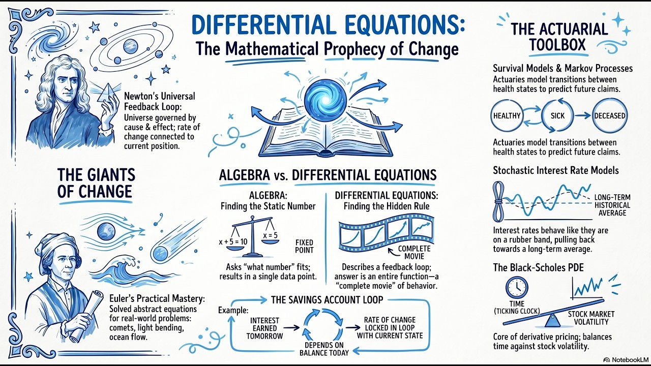
The video begins by contrasting static photographs with dynamic reality, using a sprinter frozen in mid-race as an analogy for how traditional algebra and standard mathematics often fail to capture motion. While a snapshot provides precise location data at a single moment, it strips away the vector of speed and direction, leaving us blind to what happens next. This limitation historically trapped humanity within isolated snapshots until Sir Isaac Newton revolutionized science by realizing that the universe operates on continuous chains of cause and effect rather than static states. By linking an object's current position directly to its rate of change in velocity through gravity, Newton created a framework where knowing the present state allows for the calculation of future destiny, effectively turning mathematics into a predictive engine capable of describing motion itself.
Building upon this foundation, the discussion highlights how Leonhard Euler transformed these abstract concepts into practical tools by developing numerical methods that could solve complex feedback loops even without visual aids, such as when he calculated planetary orbits while blind. The core distinction between standard algebra and differential equations is then illustrated through a savings account example: whereas algebra yields a single static number like "five," solving the differential equation for compound interest produces an entire function—a complete mathematical movie of wealth growth over time. This shift allows actuaries to move beyond simple snapshots and instead model continuous systems where today's reality dictates tomorrow's risk, enabling them to project decades into the future with confidence rather than relying on guesswork or static assumptions that would lead to financial insolvency in a changing world.
The transcript further explores specific applications of these equations across different domains, starting with human mortality using Markov models and Kolmogorov forward and backward equations to track populations flowing between health states over continuous time. It then addresses the volatility of interest rates through stochastic differential equations like the Vasicek and Cox-Ingersoll-Ross (CIR) models, which incorporate a "rubber band" mechanism known as mean reversion to prevent unrealistic outcomes such as infinite negative rates. Finally, the video examines equity markets using the Black-Scholes partial differential equation, explaining how it balances deterministic time decay against stochastic stock price movements by constructing riskless portfolios through continuous hedging, thereby transforming derivative pricing from an art into a rigorous engineering discipline grounded in the mathematics of destiny.
In conclusion, the episode emphasizes that while differential equations provide flawless mathematical frameworks for predicting futures based on current conditions, their accuracy is fundamentally constrained by the precision of our initial observations and assumptions. A tiny error in measuring today's mortality rates or market volatility can compound exponentially over time due to the nature of continuous feedback loops, leading to completely wrong predictions despite perfect mathematics. The video ends with a sobering reminder that an actuary's ability to protect society from future risks—whether demographic shifts, inflation spikes, or market crashes—is only as reliable as their understanding and measurement of the present moment, urging students to appreciate both the power and the inherent limitations of these predictive tools in safeguarding financial promises.
Read the full video transcript
You know, when you look at a a really
high resolution photograph of a sprinter
right in the middle of a race, you get
this incredible amount of specific
information.
>> Oh, yeah. Like the exact muscle tension,
>> right? Exactly. You see the tension in
their quadriceps. You see the angle of
their torso or, you know, exactly where
their foot is hovering just like a
millimeter above the track.
>> Totally frozen.
>> Yeah. It's a flawless snapshot of a
single frozen moment in time. But the
thing is that photograph is essentially
lying to you.
>> I mean, it implies a stillness that
completely contradicts the reality of
what's actually happening.
>> Exactly.
>> Because you looking at a system that is
defined entirely by motion, but you're
viewing it through a medium that is just
well stripped all the momentum away.
>> Right. It gives you a really precise
location, but it completely robs you of
the vector.
>> Yeah. You lose the direction and the
speed. I mean, from that one static
image, you can't actually tell if the
sprinter is accelerating toward the
finish line or if they've uh just pulled
a hamstring and are in the split-second
process of collapsing
>> or if they're just doing a slow warm-up
jog, really,
>> right? You have a position, but you are
completely blind to what happens in the
very next second. You just have no idea
what the future holds.
>> And mathematically speaking, for a
massive portion of human history, we
were basically trapped inside that
photograph.
>> We really were. We were operating in
this world of static numbers and
isolated snapshots. I mean we could
measure where things were but we
completely lacked the language to
calculate the mechanics of the motion
itself.
>> So welcome to all of you listening
whether you are an actuarial student who
is just deep in the trenches of exam
prep or uh simply someone who is
insanely curious about how the hidden
mechanics of reality are calculated. We
are taking a massive step forward today.
A really big step.
>> Yeah. Think about the mathematical road
we've traveled together so far in these
deep dives. We started at the absolute
beginning, right? Building the universe
from scratch with sets,
>> right? The fundamental atomic structure
of logic.
>> Exactly. We use sets to establish the
basic parameters of existence. And then
we powered that universe up.
>> We introduced functions.
>> Yes. We created these rigid predictable
relationships between different
elements. And we learned how to measure
the sheer instantaneous speed of those
relationships using differentiation,
>> which is huge,
>> right? And then we figured out how to
accumulate their total weight and mass
over [clears throat] time using
integration. We even found the rhythm,
like the literal footsteps of the
logical universe, using sequences and
series.
>> And those are all incredibly powerful
tools. I mean, you can't do modern math
without them.
>> Definitely. But everything you just
described, differentiation, integration,
functions, those are essentially just
the components of an engine sitting on a
workbench.
>> Ah, okay. I like that analogy.
>> Yeah, they are the gears, you know, the
pistons, the spark plugs. But today, we
are putting the engine together. We are
turning the key and we're actually
driving.
>> I love that. Okay, let's unpack this.
Today, we are diving into differential
equations. And I really want to frame
this for you not just as another hurdle
on a syllabus or, you know, another
chapter in a textbook.
>> It's so much more than that.
>> It really is. It is the ultimate
predictive tool in all of applied
mathematics. This isn't just about
finding the slope of a curve.
>> No, not at all.
>> This is literally the written prophecy
of change. It is the mathematical
framework we use to calculate destiny.
>> That's a bold way to put it, but it's
completely accurate. And to understand
how actuaries use this machinery today,
like to project financial risk decades
into the unseen future, we have to
understand the philosophical shift that
birthed it.
>> Right. We have to go back.
>> Yeah. We have to rewind to the late
1600s and look at Sir Isaac Newton
because Newton didn't invent calculus
and differential equations just for the
sake of like academic publishing.
>> He wasn't just trying to get tenure,
>> right? He built them because the
existing math of his era was completely
failing him. It couldn't solve the
greatest mystery of his age,
>> which was the movement of the heavens. I
mean, for most of human history, looking
up at the night sky meant looking at
this beautiful but kind of terrifying
chaos.
>> It was just dots of light moving in
weird patterns.
>> Yeah. But eventually, astronomers like
Kepler managed to map out that the
planets actually orbited the sun in
these perfect predictable ellipses.
>> Kepler did incredible work. He had the
geometry down perfectly.
>> He did. that he had the photograph to
use our earlier analogy.
>> Exactly.
>> Yeah.
>> Kepler could tell you what the planets
were doing. He could describe the shape
of the track the sprinter was running
on. But the why was completely missing,
>> right? The hidden engine.
>> Yeah. Nobody knew the hidden engine that
was forcing the planets along those
specific elliptical paths. And that's
where Newton comes in. He realized
something that completely shattered the
scientific paradigm of the 17th century.
>> What was the main realization? He
realized that the entire universe is
governed by a continuous unbroken chain
of cause and effect.
>> Okay, a continuous chain. So he
theorized that if you know exactly where
a planet is right now at this precise
millisecond and you know the
mathematical rule for how the sun's
gravity is pulling on it, you can
calculate exactly where that planet will
be 1 millisecond from now.
>> Yes, you don't need a telescope to see
the future anymore. You just need the
mechanics of the change. That is just
wild.
>> It's a huge conceptual leap. He realized
that the rate at which the planet's
velocity changes, which is its
acceleration, is directly dictated by
its current position relative to the
sun.
>> Okay. Wait, let me make sure I have this
sequence right. The position dictates
the gravitational pole.
>> Right.
>> And then the pole dictates the
acceleration.
>> Exactly. And the acceleration updates
the velocity,
>> which in turn updates the position. It's
a continuous closed feedback loop.
That's exactly it. A continuous feedback
loop.
>> But you know, capturing a continuous
loop in a mathematical formula seems
like a paradox.
>> How so?
>> Well, standard algebra demands that an
equation balance out to a static value,
right? Like x= 5. But if gravity is
constantly pulling and the planet is
constantly moving in response to that
pull, the inputs are changing infinitely
fast.
>> Did it ever start changing?
>> Right? So instead of writing an equation
that equals a static number, he wrote
one where the rate of change is directly
connected to the current position.
But how does a mathematical feedback
loop actually play out in real time? How
do you write an equation that updates
itself simultaneously?
>> Well, the trick is you have to abandon
the search for a static number entirely.
>> Okay, so no more x= 5,
>> right? You write an equation where the
variables represent the rates of change
themselves. A differential equation
doesn't say position equals x. It says
the change in position is equal to this
function of the current position.
>> Oh, I see. It is a dynamic statement of
causality.
>> Exactly. The change happens because of
the position and then the position
changes because of the change. And this
is all happening simultaneously across
infinitely small slices of time.
>> Which brings us to the 1700s and a man
who took Newton's foundation and
basically built a skyscraper on top of
it.
>> Ah, Leon Hard Oiler. Yes, Leon Hard
Oiler, a Swiss mathematician, incredibly
prolific, and arguably one of the
greatest analytical minds to ever exist.
>> He really was. Oiler is the one who
truly mastered the mechanics of these
feedback loops.
>> He took the theory and made it workable.
>> Yeah, he developed brilliant numerical
methods for taking these highly abstract
differential equations and actually
solving them to track real world
phenomena. And the detail about Oiler
that always just underscores the pure
logic of this math for me is that later
in his life he went completely blind.
>> It is an incredible story.
>> He lost his sight entirely. Yet his
mathematical output actually increased.
>> Which sounds impossible until you
understand how he thought because a
differential equation is a pure logic
system of cause and effect. He didn't
need to physically see geometric shapes
drawn on parchment anymore.
>> He could hold the dynamic feedback loop
entirely in his mind. Exactly. He could
calculate complex planetary orbits like
the Nbody problems involving the
gravitational tugof-war between the sun,
the earth, and the moon completely in
his head.
>> Just mentally keeping track of all those
moving variables.
>> Yeah. He would mentally process the
current positions, calculate the
simultaneous rates of change, update the
positions, and run thousands of mental
iterations in the dark.
>> That is all inspiring. taking these
abstract equations and finding real
world applications. He was using
differential equations to track comets
screaming through the solar system.
Right?
>> Comets, the bending of light through
lenses, even the chaotic fluid dynamics
of ocean currents.
>> He basically proved that the mathematics
of the heavens scaled perfectly down to
the physical chaos of the earth. The
rules of continuous change are
universal.
>> They absolutely are. Which brings us
directly to your world listening to this
today.
>> Yes. Tracking a comet is great for an
astronomer, but how do we translate this
cosmic math into something you can
actually use in everyday language?
>> Well, to transition this from 17th
century astrophysics to modern actuarial
science, we have to look really closely
at the anatomy of these equations.
>> We need to see the gears,
>> right? We have to clearly delineate the
boundary between the math you learn in
high school and the math you use to
price a 30-year annuity.
>> Okay, let's do it. Think about standard
algebra. We need a baseline here.
>> Sure.
>> Algebra asks a very direct limited
question. It basically asks what number
when multiplied by two equals 10.
>> And the answer is five.
>> Right? The answer is just a static
value. It doesn't tell you how that five
was created or what that five is going
to turn into tomorrow. It's just the
photograph.
>> What's fascinating here is how a
differential equation asks a
fundamentally different question. It
assumes the environment is already in
motion.
>> The clock is already ticking. Exactly.
And it asks what is the hidden rule
governing this entire changing system?
>> So the easiest way to visualize this
rule in action I think is to look at a
continuous savings account. This is the
classic actuarial starting point.
>> It's the perfect analogy,
>> right? Because if you want to know how
much interest you're going to earn
tomorrow, you look at your balance
today. Your rate of growth is
permanently locked to your current
state.
>> Compound interest is the quintessential
differential equation. The rate of
change of your wealth with respect to
time, let's just call it DWDT, is equal
to the interest rate multiplied by your
current wealth, WD.
>> So if W goes up, DWTT goes up instantly.
>> Yes. Which pushes W up even further,
>> which pushes DWT up again. It's that
locked feedback loop.
>> Exactly. And because the question is
fundamentally different from algebra,
the solution takes a completely
different form. When you solve the
algebra problem, your answer is a
number. But when you solve the
differential equation for that savings
account,
>> your answer is not a number. Your answer
is an entire function.
>> Wait, really? The answer itself is an
equation.
>> Yes, it is a complete mathematical
blueprint of the systems behavior. If
standard math gives you a photograph,
solving a differential equation gives
you the entire movie.
>> The entire movie.
>> Yeah. It gives you a continuous curve
from the moment the account was open
straight through to the end of time. You
can plug in any future date like t
equals 10 years or t equals 50 years and
the function will output the exact state
of the system at that precise moment.
>> Okay. So if the answer is an entire
movie of the system, does that mean
actuaries are essentially the movie
directors or are they just the audience
trying to guess the ending?
>> That's a great question. Actuaries
aren't the directors writing the script,
>> the universe itself.
>> Yeah. you know, human biology,
macroeconomic forces, market psychology
that writes the rules of the system.
>> The universe sets the differential
equation.
>> Exactly. The actuary is the analyst who
decodes it. They read the mathematical
script beforehand so they can prepare
the financial architecture for the twist
ending,
>> which perfectly bridges us into how
actuaries actually utilize this movie to
do their jobs. We can call this the
actuar's burden.
>> The burden of foresight really.
>> Yeah. The core duty of this profession
is to project the current state of the
world decades into the unseen future. I
mean, if you are pricing a long-term
care insurance policy or reserving for a
pension fund, you absolutely cannot rely
on static numbers.
>> You'd be bankrupt in a week.
>> Exactly. A static photograph of a
healthy 30-year-old gives you zero
actionable data about the medical
reserves you will need to liquidate when
that person is 85.
>> Because today's reality dictates
tomorrow's risk. That is the
foundational axiom of the whole field.
>> Today's reality dictates tomorrow's
risk. That is so crucial because
actuaries look at deeply interconnected
systems where one single change cascades
through time.
>> Right? If inflation ticks up by say 50
basis points this afternoon, it's not an
isolated event.
>> It changes everything. It alters the
trajectory of bond yields, which alters
the compound growth of retirement
portfolios, which reshapes the liability
profile of massive corporate pension
plans 30 years from now.
>> It's the butterfly effect, but with
money. And that's why this predictive
machinery is the absolute crowning jewel
of the actuarial toolkit.
>> It's the only mathematical framework
rigorous enough to integrate those
cascading ripples over continuous time.
It allows you to step completely out of
the present moment and confidently map
out decades of unknown risk. Okay,
here's where it gets really interesting.
Let's move from the philosophy of risk
to the exact specific scenarios where
you, the listener, will use these
equations in the field. Let's examine
the actual mathematical battlegrounds.
>> We should start with perhaps the most
complex system of all, human mortality
and morbidity. Yes, we are talking about
survival models and specifically what
the actuarial world relies on heavily
multiple state Markoff process models.
>> Right now in traditional algebra a
variable is just a placeholder for an
unknown quantity. But in a marov model a
state is a literal condition of
existence.
>> Okay. So paint a picture for us. Imagine
you are managing a massive block of
long-term care insurance policies. Okay.
You have tens of thousands of policyh
holders. At any given moment, every
single one of those individuals exists
in one of a few highly specific state,
>> right? They might be completely healthy
>> or they might transition into being sick
and requiring nursing care.
>> They might recover and transition back
to healthy.
>> Exactly. Or they might transition into
the terminal state of having passed
away.
>> Those are your states and your
population is constantly flowing between
them. But the analytical key here is
that the flow of these populations is
not mathematically random.
>> Even if an individual's health feels
entirely unpredictable to them,
>> right? The rate at which people
transition from the healthy state to the
sick state over the next continuous time
interval depends entirely on the volume
of people currently sitting in the
healthy state.
>> It's the continuous savings account
dynamic again, just applied to human
biology instead of capital.
>> The rate of change depends on the
current balance. Exactly. So to model
this flow across continuous time like to
project how 50,000 people will migrate
through these states over the next 40
years actuaries rely on a highly
specialized set of differential
equations.
>> The famous Kaggarov forward and backward
equations.
>> Yes, Kurov. And for a student
encountering these equations for the
first time, I mean the notation alone
can look like a wall of hostile Greek
letters.
>> Oh, it's intimidating. You've got
transition probabilities, transition
intensities, matrix multiplication.
>> It's a lot. But underneath all that
heavy notation, what exactly is the
mathematical engine doing?
>> Fundamentally, they are tracking the
continuous rate of change of
probabilities.
>> Yeah,
>> let's break down the mechanics.
>> Let's do it.
>> The Cole McGraov forward equation does
exactly what it sounds like. It anchors
you in the present state. Say you have a
healthy 65y old today and it projects
forward.
>> Okay, so it's moving into the future,
>> right? It integrates the transition
intensities which are the continuously
changing hazard rates of getting sick or
dying to calculate the exact probability
distribution of that person being in any
specific state at time in the future.
>> So it moves from a known present to a
probabilistic future.
>> Exactly.
>> Okay. So the forward equation maps out
where the population is going to end up.
What does the backward equation do? The
backward equation is the actuar's
ultimate reserving tool. It flips the
temporal perspective entirely.
>> It goes in reverse.
>> Yes. It fixes a specific payout
requirement in the future. So let's say
there's a $5,000 monthly nursing home
benefit that triggers if the policy
holder is in the sick state at age 85.
>> Okay? So we know the future liability,
>> right? The equation then works backward
through continuous time applying the
transition intensities in reverse to
calculate the exact present value of
that future liability today.
>> Okay. Wait, let me push back on this for
a second.
>> Sure.
>> If Kumagarov's equations are tracking
human health, I mean, human health on an
individual level is basically biological
chaos.
>> It definitely is.
>> A perfectly healthy person could get
into a catastrophic car accident
tomorrow or a sick person might receive
an experimental treatment and fully
recover. So, how does a deterministic
differential equation turn that kind of
unpredictable biological chaos into a
reliable, legally binding 40-year
financial projection?
>> It seems like it shouldn't work,
>> right? Doesn't the rigid math break down
the second humans start acting like
humans?
>> That is the exact conceptual hurdle
every single actuarial student has to
clear. But the math does not break down
because the differential equation inside
a Markoff model does not care about the
individual.
>> Oh, interesting. It is engineered to
operate on the aggregate.
>> Ah the law of large numbers.
>> Yes. But applied continuously. On a
micro level, health is stochastic. It is
a random walk. But when you aggregate
50,000 policy holders, the variance of
that random walk compresses.
>> The noise cancels out.
>> Exactly. The biological chaos smooths
out into highly predictable continuous
transition intensities. So by solving
Colgrav's backward equation, an
insurance company isn't trying to guess
the fate of John Smith. They are
calculating the mathematical expectation
of the entire risk pool.
>> So that so what insight here is the
power of large numbers in these feedback
loops. By solving that equation today,
they know down to the dollar how much
capital they need to hold in reserve to
guarantee those claims in 2055. Yes,
they are using the exact same continuous
feedback loops that Oiler used to track
planetary momentum but applying them to
ensure a portfolio remains solvent
through decades of human aging.
>> That is just brilliant. But human health
is just one type of unpredictability and
it has a distinct mathematical advantage
for an actuary, right? You eventually
decays in a predictable direction. Yes,
morbidity rates generally increase with
age and mortality is well a certainty.
The variables have biological limits,
>> right? Which brings us to a massive
pivot. What happens to our predictive
machinery when the variable we are
tracking has no biological limits?
>> When it can move in any direction at any
time.
>> Exactly. Driven entirely by human
psychology and macroeconomic pressure.
We need to move from human biology to
financial mathematics. We need to talk
about the continuous movement of
interest rates.
>> This is where things get really dynamic.
Yeah,
>> because when you first learn about the
time value of money, you basically treat
the interest rate as a constant,
>> right? In Exam FM, early on, a bank
offers a 5% yield. You plug it into your
discount factor formula and you discount
your cash flows.
>> It's static. But in the real world of
institutional finance, pricing a 30-year
bond portfolio based on a static
interest rate is just financial suicide.
>> Because interest rates do not sit still.
They wander. They jitter continuously
based on inflation data, central bank
announcements, global liquidity,
everything.
>> They exhibit stochastic behavior. They
follow a random walk over time.
>> But it's not a pure random walk, is it?
>> No, it's not. Because if an interest
rate were purely uniformly random, it
could mathematically drift up to a
million% or plunge to negative 5,000%.
And that obviously doesn't happen. The
economic environment restricts it.
>> Exactly. Interest rates are tethered.
They exhibit a property known as mean
reversion.
>> Meaning they have this deeply ingrained
mathematical tendency to pull back
toward a long-term historical average.
>> Right? And the classic physical analogy
here is a heavy rubber band.
>> Oh, the rubber band analogy is perfect
because the daily volatility of the
market is constantly pushing the
interest rate around, right? It's
stretching the rubber band
>> up and down. But if rates drop too low
for too long, inflationary pressures
build up, capital tightens, and the
rubber band violently snaps the rate
back up toward the equilibrium.
>> And conversely, if rates spike too high,
the economy chokes, borrowing stops, the
central bank intervenes, and the rubber
band pulls the rate back down.
>> It is a continuous tugof-war between
random volatility and the magnetic pull
of the mean. And to capture that exact
tugof-war, actuaries use stochastic
interest rate models. The foundational
examples being the Vasich model and the
Coxinger Ross model. Yeah. Widely known
as the CIR model.
>> Right. And these are built entirely on
differential equations. But to capture
both the randomness and the rubber band,
you can't use standard calculus.
>> No. Standard calculus assumes
deterministic smoothness.
>> You need a formula that calculates the
tension of the rubber band at any given
millisecond while simultaneously
accounting for the random shocks. You
need a sootastic differential equation.
Let's look at the mechanics of the
Vasich model first. Yeah,
>> it defines the instantaneous change in
the interest rate which we call dright.
>> And it splits that change into two
distinct components.
>> Okay. What's the first component?
>> The first component is the drift term.
In the formula, it's a time B minus or
T.
>> That's the rubber band. B is the
long-term average rate. R is the current
rate. And A is the speed of reversion.
Like how thick and tight the rubber band
is.
>> Exactly. So if the current rate or t is
way below the average b that term
becomes highly positive forcefully
pulling the rate back up.
>> Okay. So that is the deterministic part
of the differential equation. But then
vasiche adds the second component
>> the diffusion term
>> right sigma time dwt where sigma
represents the volatility and dwt that
is a wiener process
>> also known as brownie in motion. This is
the mathematical engine of randomness.
It represents the unpredictable
continuous wiggling of the market noise.
>> Okay. So, if these models describe a
random drifting combined with the
magnetic pull of the average, which
force usually wins out in a 30-year bond
horizon? The randomness or the magnet?
>> Well, if we connect this to the bigger
picture, the stochastic differential
equation perfectly balances these two
forces over time.
>> Oh, so
>> over a short window, say a 3-day period,
the wiener process, the random noise
completely dominates the equation. the
rate just jitters unpredictably.
>> The magnet isn't strong enough over
three days,
>> right? But integrate that equation over
30 years and the drift term, the rubber
band, really asserts its dominance. The
math allows you to price the long-term
tension of the market, generating the
exact yield curve you need to value
future liabilities accurately.
>> But the faucet model isn't flawless, is
it?
>> No, it has a pretty significant quirk.
Because the wiener process is normally
distributed, the random shocks can
theoretically push the interest rate
below zero.
>> The math allows for negative interest
rates,
>> which historically speaking was
considered a major flaw in the model.
>> Which is exactly why the Coxing Ross
model, the CIR model was developed as an
evolution. It takes the Vasich
differential equation and makes one
brilliant mechanical tweak.
>> It multiplies the volatility term by the
square root of the current interest
rate.
>> Why the square root?
>> Think about the behavior. As the
interest rate drops closer and closer to
zero, the square root of that rate also
approaches zero.
>> Oh, I see.
>> This effectively shrinks the volatility
term. The closer the rate gets to zero,
the weaker the random shocks become,
while the upward pull of the rubber band
remains strong.
>> So, the differential equation
mathematically builds a floor. It
prevents the random walk from crossing
into negative territory.
>> It's an incredible piece of financial
engineering.
>> It really is. You are tweaking the
parameters of a differential equation to
alter the fundamental physics of this
simulated economy.
>> We're setting the rules of the universe.
>> Yeah. Okay. So, we've used Marov models
to map the biological decay of human
populations. We've used Vasich and CIR
to tether the random walk of macro
interest rates, but we've protected
human health in interest rates. There is
one more volatile frontier that requires
the most famous equation of them all.
the most volatile, chaotic and
relentlessly measured environment on
earth, the equity markets.
>> Yes, we are moving into financial
economics and the valuation of
derivatives, the crown jewel of finance.
>> If you want to price a financial option,
let's say a European call option, which
gives you the right to buy a specific
stock at a specific price on a specific
date in the future, you are trying to
price a moving target based on another
moving target,
>> which is incredibly hard. You cannot use
arithmetic. You have used what is widely
considered the most famous equation in
modern quantitative finance, the black
skulls formula.
>> Yes, black skulls. But I want to unmask
black skulls here because what many
students fail to grasp when they first
memorize the formula is its true nature.
>> It looks so static on the page,
>> right? When you see black schools
printed in a study manual, it looks like
this massive static algebraic formula
involving cumulative normal distribution
functions D1 and D2. You plug in the
stock price, the strike price, the time
to expiration, the risk-free rate, and
the volatility, and boom, the formula
spits out the fair value of the option.
>> But that massive formula is just the
closed form solution.
>> Exactly. It is just the final photograph
of the sprinter crossing the finish
line. The algebraic formula is just the
aftermath. At its absolute fundamental
core, Black's goals is a partial
differential equation.
>> A partial differential equation. We have
leveled up again. Meaning there isn't
just one variable changing over time.
There are multiple independent variables
changing simultaneously. And the
equation is rigorously tracking how
their respective rates of change
interact with each other. In the case of
an equity option, its value is
constantly shifting, but it is being
aggressively pulled by two entirely
different forces simultaneously.
>> Let's break down the mechanics of those
two forces. On one side, you have the
passage of time,
>> the ticking clock,
>> right? Every single second that ticks
by, the option gets closer to its
expiration date. This creates time decay
or what options traders call theta. Time
only moves in one direction. It is a
relentless, smooth, deterministic decay.
The partial derivative with respect to
time is easily knowable.
>> But on the other side, you have the
underlying stock price.
>> Yes, the unpredictable volatile
wiggling.
>> The underlying asset is moving
stochastically.
It is jumping up on earnings reports,
crashing on supply chain rumors,
wiggling constantly.
>> And this volatility affects the options
value traders call the rate of change
with respect to the stock price delta.
And the rate of change of delta itself,
Gamma.
>> Exactly. So the partial differential
equation of black's goals is trying to
reconcile the perfectly smooth
deterministic decay of time against the
violently unpredictable stoastic
wiggling of the stock price.
>> Okay, wait. Can a partial differential
equation actually tame the volatile
wiggling of the stock market? Or does it
just give us a very accurate measurement
of how dangerous that wiggling is? How
do you possibly balance those two
things? You balance them by applying
Ido's lema which is a cornerstone to
stochastic calculus. Yeah. To construct
what is known as a riskless portfolio.
>> Riskless portfolio.
>> Yes. Black Scholes and Merin realized
that if you continuously buy and sell
the underlying stock in a very specific
ratio to the options you hold, a ratio
dictated by the differential equation
itself, the random wiggling of the stock
price perfectly cancels out the random
wiggling of the option value.
>> Wow. So the DWT, the wiener process
representing the random noise is
mathematically eliminated from the
equation.
>> Precisely. You have hedged away the
market risk entirely.
>> And if the portfolio has zero market
risk, economic theory dictates that it
must grow at exactly the risk-free
interest rate.
>> That is the genius of the black skulls
partial differential equation. It
equates the continuous hedging of the
option to the risk-free growth of cash,
allowing you to solve for the exact fair
value of the derivative. today.
>> A great way to visualize this isn't
trying to put the beast of the market in
a cage because nothing tames the market,
right?
>> The market is driven by infinite human
fear and greed.
>> You can't control it.
>> Instead, think of the black skulls
equation like a massive continuously
spinning gyroscope installed deep inside
the hole of a cargo ship.
>> Oh, I like that. The ocean is the market
volatility,
>> right? The gyroscope does not calm the
ocean. The waves are going to crash.
Storms are going to hit. Black swan
events are going to generate massive
swells. It just accepts the chaos.
>> Exactly. But the differential equation
inside that gyroscope is continuously
calculating the roll of the ship, the
angle of the waves and instantaneously
adjusting the mechanical stabilizers. It
mathematically offsets the chaos of the
environment so that the cargo, the
portfolio's core value remains perfectly
level.
>> And the profound nature of discovering
that specific partial differential
equation cannot be overstated. It didn't
just earn a passing grade in a
quantitative finance seminar. The
conceptual framework won a Nobel Prize
in economics.
>> It's that huge.
>> It transformed the valuation of
derivatives from an esoteric guessing
game into a rigorous engineering
discipline. It literally catalyzed the
creation of the modern global
derivatives market, a system that
manages hundreds of trillions of dollars
in notional risk.
>> That's staggering.
>> The entire global architecture of
financial hedging rests securely on the
mathematics of continuous change. Which
brings us to the ultimate synthesis of
our deep dive today. What we have been
exploring for the past hour is not just
a collection of formulas to be memorized
for an actuarial exam.
>> No, it's so much bigger.
>> We are talking about the mathematics of
destiny. Differential equations are the
precise tools that allow us to isolate
the hidden rules of cause and effect
operating in the present moment to
financially protect the reality of
tomorrow. We observe the system. Whether
it is a planet trapped in gravity, a
human population aging through a marov
chain, a macroeconomic rubber band
snapping interest rates back to the
mean, or a gyroscope hedging the chaos
of equity markets.
>> We identify the dynamic feedback loop
governing their continuous change.
>> And by solving that equation, we map out
the architecture of tomorrow. So if you
are an actuarial student listening to
this, I know it is incredibly easy to
get buried in the notation, to stare at
a page full of partial derivatives,
wiener processes, and transition
intensities and completely lose the
narrative plot.
>> It happens to everyone. But if you
connect the grand historical visions of
Newton staring at the perfect ellipses
of the night sky and oiler calculating
planetary momentum in the dark to your
daily practical reality, it elevates the
entire profession. You aren't just a
financial accountant crunching static
numbers.
>> You are the operators of this predictive
machinery. You are the engineers tasked
with protecting the future.
>> That is exactly right. You utilize these
equations to ensure that when the future
actually arrives, whether it brings a
demographic shift in mortality, a
massive inflationary spike in interest
rates, or a catastrophic equity market
crash, the financial foundations of
society do not buckle.
>> You use the math of destiny to ensure
that the promises society makes to its
citizens are actually kept.
>> It's a huge responsibility.
>> It is. And as we wrap up, I want to
leave you with one final sobering, maybe
provocative thought about the mechanics
of this prophecy. We have spent an hour
establishing that a differential
equation gives you a perfect
mathematical movie of the future driven
entirely by the rules of cause and
effect applied to the present state of
the system.
>> Right? The initial conditions, the
values you plug in at time zero.
>> Exactly. The equations themselves,
Kaggarov, Vasich, black skulls are
mathematically flawless. But if a
differential equation gives you the
perfect movie of the future based
entirely on the conditions of today,
what happens to the actuar's 30-year
prophecy? If our measurement of today is
off by just a fraction of a percent.
>> Ah, that is the danger. The nature of a
continuous feedback loop is that errors
do not remain static.
>> They grow. In a dynamic system, a tiny
miscalculation in the initial conditions
is fed back into the equation, amplified
by the rate of change, and fed back in
again. The error compounds exponentially
over a continuous time.
>> So, if the initial mortality assumption
fed into the Marov model is off by just
a little bit, or the estimate of current
market volatility is slightly skewed,
the flawless mathematics of destiny will
perfectly calculate the completely wrong
future.
>> The math is perfect, but the starting
line isn't
>> right. The math of destiny is flawless,
but how perfect is our starting line?
So, as you push forward in your studies,
as you master the rigorous equations of
continuous change, never forget that
your ability to project decades into the
future is fundamentally constrained by
your precision in observing the present
moment.
>> Your mastery of tomorrow is only as
reliable as your understanding of right
now.
>> Keep pondering that. Keep exploring.
Keep questioning the mechanics of the
systems around you. And we will see you
on the next deep dive.