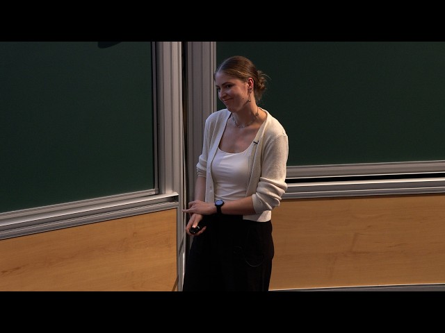
Anna Wolz - Gravitational Scattering off Compact Objects from Partial Waves

Okay. [music] Thank you. Thanks to the organizers for a great conference and uh giving me the opportunity to talk. So yeah, today I'll be talking about some work that came out um this past summer with my collaborators Miguel Koreah and Julia Isabella on the gravitational scattering off of compact objects from partial wave space. So the motivation for why we care about gravit gravitational scattering here is of course you know 10 years ago uh with the first discovery of gravitational waves ushered in a new era of gravitational wave astronomy allowing us to understand the dynamics of objects in our universe based on the gravitational wave radiation they uh gravitational wave emission that we detect with our detectors. So for a long time [snorts] at the beginning of the signal you have two objects typically orbiting around each other in a binary that emit gravitational wave radiation that for a very long time with a very slowly varying signal. Eventually the objects get closer and closer together. You get to start to see different kinds of effects. Gravity gets stronger as they get closer together. Eventually the objects merge in a very nonlinear violent fashion. And then after they've merged, you're left with one object ringing down just like after a bell has been rung you know emitting radiation as it uh rings down to equilibrium. So we have you know kind of truth to uh describe exactly what this signal looks like. It's called numerical relativity and we use this to describe the highly nonlinear part of our signal that happens during the merger because it's too complicated to try to do perturbation theory there. The downside is that numerical relativity is very computationally expensive. So we don't want to spend too much time uh in terms of our signal using numerical relativity. So we need analytic methods to describe both the inspiral and the ring down. One very powerful uh analytic tool that we have is effective field theory. So in the inspiral when your two objects are very far away from each other they're approximately point particles. When the typical separation distance is much larger than the size of either of the objects you can approximate them as points in space. You can write down in uh effective field theory for example just some masses at a point in space. Um in addition to using effective field theory a very very powerful tool that we have is to use scattering amplitudes as we heard today. So uh thankfully Stephano and Jungwuk gave a nice introduction to this but the basic idea is we can use scattering amplitudes in an appropriate classical limit. So here I write it as inudes of h bar equals 1 large angular momentum in our system. So the uh typical separation distance between the objects times our momentum is much greater than one. And in this limit you can uh imagine a scattering experiment where you scatter two massive scalers off of each other. These straight lines here they exchange gravitons and this tree level exchange you can show that you can compute the Newtonian potential between two objects. Now this Newtonian potential has general relativistic corrections at higher order in G and you can get those from the classical limit of loop diagrams. So in this talk when I talk about loops I'm usually talking about higher order in uh gon general relativistic corrections. So this has been uh these you know twopoint particles in vacuum has been uh studied extensively from the amplitudes community to compute correct GR corrections to in spiral dynamics for example. But in today's talk I'm going to focus on uh basically an extension of this effective field theory. In this point particle effective field theory, you can extend it to include higher dimension operators. And these higher dimension operators encode finite size effects that can show up in your system. So I have some twopoint particles. As they get closer together, they start to deviate from this point particle approximation that we've made. These deviations are encoded in what are called uh love numbers. They can describe for example the title deformability of the object. So in the presence of some gravitational field your object is no longer a perfect sphere. It has some uh you know feels the effect of the tides or additionally uh dissipation as well. So I've drawn here is just an example higher dimension operator that corrects the effective field theory. This emu is some component of the vile tensor. I'll describe it in a little bit more detail later. But the Wilson coefficient in front of this operator is called a uh title love number. Now these love numbers have been studied for a long time from many different perspectives. Uh for the specific case of a black hole. So I have some generic object and the love number takes different values depending on what that object is. For the specific case of a black hole, it was shown that uh the static love numbers are zero for black holes. Um have been shown recently. There's been a lot of interest in uh arguing this from different symmetry perspectives. But anyway, very interesting things to study. Now, this is a two-body setup where finite size effects enter. We'd like to study them from a bit of a more simplified scenario, which we can do because finite size effects also show up in the ring down phase. So, I have one object emitting gravitational wave radiation and you can uh see the deviations from the point particle approximation during the ringdown phase as well. So let me zoom in now on the ringdown. You can model the ringdown as a wave scattering against some static background that's sourced by your object. For the specific case of a black hole, this is nothing new. This is what's called black hole perturbation theory. The basic idea is you write down the short chilled metric sourced by your object plus some massless perturbation on top of it. You can derive the equation of motion for this massless perturbation. And since my uh system is spherically symmetric, I'm just considering Schwarzfield here and no spin. So since this situation is spherically symmetric um you can show that the equation of motion for this perturbation reduces to a one-dimensional radial wave equation at fixed angular momentum L. So trying to understand the uh emitted radiation during the ringdown just reduces to trying to solve a wave equation on some background. You can um and so we do this by studying this response object. Basically I scatter a wave against some background and I measure the response at infinity through this object. the response coefficient SL of omega at fixed angular momentum and it's really just the ratio of the incoming and out the coefficients of the incoming and outgoing plane waves here. So this object you can study it non-perturbatively um last year we showed that the uh analytic structure of this object is constrained by fundamental principles. So if I plot the response coefficient in the complex frequency plane there's two interesting analytic structures that appear. The first is this branch cut running along the imaginary axis due to the long range nature of the gravitational potential. Additionally, in the lower half plane, we have these quasormal modes that are basically particular solutions where I set the incoming coefficient to zero and these govern this exponential damping of the uh gravitational wave signal during the ring down phase and they show up as poles in the lower half plane here. Perturbatively we can um try to solve this differential equation and get explicit results in the regime where the Schwarz shield radius o is much smaller than the wavelength of my uh scattered wave and so in this regime GM omega much less than one you can use various methods for example MST to solve this wave equation perturatively so this is for the case of a black hole but what if I don't care about a black hole and I just want to study some uh generic object. So I have my point particle. You have a question. >> Yeah. So how does the the previous slice differ from the known previous results? I mean this >> Yeah. No, no, yeah. Yeah. This is this is mostly known what we showed last year specifically um that this branch cut rungs along the entire half um entire imaginary axis. For example, people knew that in the greens function, which is maybe a more natural object that people study in black hole perturbation theory, there's this branch cut that runs in the lower half plane. Whereas this object, which as we'll show, you can relate to a scattering amplitude, has this branch cut running in the upper plane. Yeah. Yeah. Now, this is Yeah. This is a lot of this is in the literature already. So the question for today's talk is can I calculate this response coefficient from my point particle effective field theory. So not specifically the case of a black hole but I can calculate this for some generic object if I could that uh this response coefficient will depend on the tidal love numbers in my theory. And so if I then match my effective field theory response coefficient to the result from black hole perturbation theory which is basically my you know UV complete theory here then I could derive the gauge invariant love numbers for a black hole. So what has been done in terms of calculating this response coefficient for a generic object? There's kind of two main approaches that you could do. First from uh the point particle effective field theory as is the case for binary dynamics you can do a fineman diagrammatic expansion to calculate the scattering amplitude a. So a depends on the frequency of the scattered wave omega and x which is some variable related to the um scattering angle and using traditional methods this has been calculated just this year to um four loops. So g to the 5 is a four loop calculation which is very impressive. Alternatively, some of my collaborators showed um in the past couple years that you can borrow ideas from black hole perturbation theory to directly calculate this object in um partial wave space. So basically what it boils down to is you take your point particle effective field theory, you project it onto a wave equation, then you solve that wave equation order by order. So very similar to black hole perturbation theory and this is a very powerful method because unlike in the scattering amplitude direct calculation each loop order is harder and harder to do generically whereas here you can kind of go to arbitrary order and perturbation theory with no more difficulty. So it's a very powerful method uh that they showed as proof of concept for the case of a scalar wave scattering. So let me just motivate this a little bit more. If you calculate this scattering amplitude in momentum space as a function of this x and omega somehow you need to match it in partial wave space if you want to say extract the black hole love numbers. So in order to do that you just project your scattering amplitude onto partial waves. So it's just a one-dimensional integral. you have a leandre polinomial uh PL cosine theta and from that you can extract this response coefficient at fixed angular momentum L. The alternative method is by solving by rewriting your Fman diagrammatic expansion as a Borne series and solving the corresponding wave equation you directly get the result in partial wave space. So the matching is you just kind of get it for free. Now this idea of [snorts] um recasting your scattering setup into a born series and solving a wave equation has been used uh since then to much success. For example to calculate this is jumping ahead a little bit but to calculate the running of the title love numbers to calculate for example cur love numbers and to calculate for example corrections to a waveform. So just to say that this method uh yeah shows a lot of promise for being able to do um uh perturbative calculations very very efficiently in a wider array of different arenas. So if we have a new powerful tool that allows us to do precision calculations to very high order. The question that I'll address in today's talk is can we use our information here to reconstruct our actual scattering amplitude. In theory, this looks like a very simple sum. You just sum over partial waves. You have your Leandre polinomial showing up here to extract this coefficient here. And I will show you today that you can indeed do it. I don't know if you'd call it simple, but you can do it. Just to motivate this a little bit more, other than saying okay, we can do this thing. I would say big picture if you want to take a step back you know a scattering amplitude as Stephano mentioned at the beginning it's naturally like a quantum field theory object it has a lot of information here about our you know high energy theory and so maybe you say okay it's straightforward to take some quantum thing and project it in the classical limit onto a much simpler setup partial ways for example you might be familiar with them from a quantum mechanics class some classical scattering setup Additionally, uh non-perturbative bootstrap methods typically are sometimes formulate things in terms of partial wave space because unitarity is very simple in that space. But anyway, so just to say that you know this problem of going from this partial wave space to the actual scattering amplitude of momentum space. It's a very very old problem. People have been working on it for hundred years. And so this is kind of the bigger picture of uh what I'll be talking about today. But for now, I'm just going to focus on how we actually reformulate our effective field theory um into a wave equation. So just to describe this EFT very generally, I have some object sitting in space with some radius R and I'm going to scatter a wave against it. And our effective field theory is going to live in the regime where the wavelength of our wave is much larger than the radius of the object. This object could be a black hole, could be a neutron star. So maybe it has some short radius that's different, but okay, we're we're agnostic about that. So if the wavelength of the wave is much larger than the radius of the object, the wave can't resolve the internal structure of the object. It effectively just sees a point of mass sitting at the origin. This is why it's a point particle effective field theory. All of the information that encodes the short distance effects living at the surface of the object as you get closer to the object is recast in terms of these uh love numbers. So the short distance physics we've expanded it away and instead we have these love numbers that enter as higher dimension operators in our theory. So this is the scales of the system that we'll be working at. So let me write down our action. Our action has three main components. First the Einstein Hilbert action governing governing dynamical gravity here. The point particle sources some short chilled background that we'll be expanding about. But remember we're at a long you know a large distance approximation. So you should really think of this short chilled background as expanded perturbatively in G. And we'll study metric perturbations on top of this background. The short distance physics as I mentioned on the previous slide is encoded in the love number contributions. So you have an infinite tower of higher dimension operators showing up in your action. We decompose them uh this is just a choice but we decompose them into um specific components of the while tensor what are typically called the electric sector and the magnetic sector. Just two parody sectors uh that you can compose these tens these um operators into. So that's why we have E and B and the coefficient in front of these operators will be the love numbers. So we have electric love numbers and we have magnetic num love numbers. >> You are in four dimensions here. >> This is in general D just for simplicity. I just wrote the action in four but yeah we we set it up in general D. So as I mentioned we have an infinite tower of these constructed from higher uh spatial and time derivatives of these operators. Basically you can rewrite all of these operators in a basis where the angular momentum L is just a number that counts how many spatial derivatives you have and this number n calculates how many time derivatives you have. And so if you've heard people talk about static love numbers, for each fixed L, the static love number is the one that has N equals Z. So it doesn't scale with the frequency. And anything beyond that is called a dynamical love number. And again, I I don't show it here, but if you use the in informalism, you can get both the conservative and the dissipative response. So the last part of this action is this point particle piece. So we just have our massive object at its world line. And you can show that if you integrate out world light fluctuations uh about this particle's trajectory, you get this recoil piece here. And so both the point particle part of my action and the love number part of my action are supported at the world line of the object. So now that we have our action, we're going to derive our effective wave equation. So I'm just going to sketch it here and not really show too many details. The basic idea is you vary your action with respect to yurometric perturbation. You project the resulting tensor onto tensor spherical harmonics. So just a generalization of uh yeah projecting it in uh due to spherical symmetry with a convenient gauge fixing choice you can show that um you reduce to basically two degrees of feed freedom um in four dimensions. So we have two master fields, one for the electric par and one for the magnetic par at fixed angular momentum. So here's my wave equation. Again, it's just some radial wave equation where I have uh in the presence of a background potential where my potential comes directly from these three pieces of my action. So what does this potential look like? while the gravitational piece just uh comes from the long distance physics encoded in that short background we perturbed about. So at large distances and ex it's an expansion in GM over r much less than one. So as I mentioned on a couple slides ago you know the all of the information about the horizon or the surf of the surface of the object has been expanded away. So this is the you know short potential contribution but since it's expanded at large distances you lose that information about the internal structure of the object. The love number piece contributes short distance physics. I mentioned on the previous slide it's only supported on the the world line of the object. When you derive the contribution to the potential here what that means is that it comes with this delta function of r. So this contribution really just lives at the location of my point particle. So it has this delta of r here and the coefficient is just uh different combinations of the love numbers. The recoil piece you can show that in dimreg the action of the recoil piece on the field uh is identically zero with this convenient gauge choice. So that simplifies our life greatly and we can just drop this recoil term. >> What is the gauge again? Uh, I think it's called Reggie Wheeler gauge. Yeah. I don't know the name, but yeah. The Yeah. >> Did they check precisely or is just that they got the right answer? >> No, no, no. We checked. >> Okay. >> They didn't. We did. >> Yeah. [laughter] Yeah. Yeah. Yes. Yeah. Yeah. Um, yeah. Basically um okay technical for a sec but the the basic idea is the at so this also comes with a delta of r contribution right it just lives at the location of the source the the solution for the wave for the wave function at small distances is powers of r and in dimrag you can show that the power of r goes with an epsilon and so it identically vanishes when you set r to zero G will is in 3 + 1 dimension not in D dimension. So >> yeah, so it's d= 4 - 2 epsilon. Yeah. So it's I I agree. But any subtleties that come with additional degrees of freedom decouple from the four dimensional degrees of freedom? No. Okay. [clears throat] So now that we have our wave equation, we'd like to solve it. So I'm going to drop a lot of in a lot of labels here, but you should think I have two copies of this equation for the two par sectors. So I can expand my solution both at small distances and at large distances. At small distances again in dimreg you can show that the long distance contribution uh vanishes which is very nice. So at short distances the only contribution we have is from v love located at the source of the object. So uh as r goes to zero the solution of this wave equation has some regular and irregular part that come with epsilons but I haven't written them out here and basically you know in a normal situation you usually impose regularity at the origin. So you usually turn off this irregular piece and you just have the regular solution. However, the presence of these delta functions living at the origin basically turn on this irregular response. And so basically by matching coefficients of the delta functions uh with different derivatives >> that it is the reverse it is r and r to the minus1us. >> Oh okay did I sorry okay typo I missed the one should go there. Sorry. Um thank you. Uh yeah so by matching coefficients of these delta functions you can fix this ratio these coefficients B irreg and b reggg in terms of our love numbers. So these love numbers basically become boundary conditions for our solution at the origin. On the other side at large distances uh at very very large distances the solution is approximately incoming and outgoing plane waves. And so we extract our response coefficient as I mentioned towards the beginning as just the ratio of the outcoming to incoming plane waves. And we'll often write this response coefficient in its exponentiated form where this delta is a phase shift. So we have our dis our solution at r goes to infinity and our solution at r goes to zero. How do we connect the two? So in between um at we're still at r greater than zero. So the love number contribution disappears and all that we have to consider is the long distance physics encoded in vgraph. So you can solve the solution order um using write a solution using a born series order by order in g you'll get different contributions from the potential and different contributions from the iterations of this born series. And basically what that gets you is this matrix that connects your solution at r goes to infinity to your solution at uh r equals z. So this connection matrix encodes all of the information about the long range gravitational effects. Uh yeah. >> So remind me here the far zone you had to iterate but in the near zone did you have to iterate on that boundary condition or was it just >> No, it's it's just fixed. Yeah. Yeah. Yeah. It's it's literally just matching um coefficients of delta functions. Yeah. So yeah, this connection matrix um in the previous paper my by my collaborators they showed that you can write it very efficiently by reorganizing these boring integrals into harmonic poly logarithms. So they're able to get this connection matrix order by order in G um very very efficiently. So the upshot is though I skipped a lot of details you can obtain this response coefficient perturbatively in G um to any order including the love number response. So I'm going to show a result on the next page. Here is an example result. So this is the phase shift for the electric par sector at fixed L equals to two. This is the first few orders in G um up through G to the 4th. You don't have any contribution from the love number. So this is purely from the long range gravitational potential. And so it's the same for any object. This looks the same for a black hole, for a neutron star, for whatever you have because the love numbers haven't entered yet. So this has been in the literature. Uh at leading order, we have the IR divergence due to the longrange nature of gravity. We have some zeta values that come from these harmonic poly logarithms that I mentioned on the previous slide. But anyway, it's just some perturbative expansion in G that you can get and this matches with the literature. At the next order in G, we have our first love number contribution. So this is the static love number at L equals 2 in the electric parody sector. At G to the 6, we have the first dissipative love number entering comes with an I. And at G to the 7, we have more love numbers that enter and we see our first UV divergence. So what is this UV divergence? This is basically telling you that um a point trying to describe a point particle in general relativity is inconsistent. The long range contribution from the gravitational potential is going to diverge at some order. And so you need some counter terms to renormalize and to remove this one over epsilon. And this these counter terms are exactly the higher dimension operators that come with title love numbers. So these love numbers here will conspire to cancel this UV divergence when you fix it to a solution. Or you can calculate the reormalization. So this is the result for the phase shift at G to the 7 where we see this UV divergence. That was kind of the first new interesting physics we wanted to see. So we stopped here. But in principle you can do this for whatever order in G if you just want to sit and wait and stare at your computer. So uh this is for our effective field theory. If we want to extract the black hole love numbers, we can match to black hole perturbation theory. And so here I've written the first few love numbers that we fixed. So these are the static love numbers at L= 2 and L= 3. We indeed see that they are zero for a black hole as expected. um this was the first dissipative love number so it just has some number and then we see that um this next dynamical love number carries this one over epsilon that will cancel the UV divergence on the previous slide so this is for the electric sector and for the magnetic sector it's approximately the same >> sorry yeah >> can you go to the previous >> thanks so in that line with the orange >> the lambda 22 with argument epsilon inverse that means the one epilon Yeah. Yeah. Sorry. That's just notation to Yeah. >> So just a leading order. >> Exactly. >> Yeah. So this plus this is equal to this. Sorry. >> Yeah. Good point. >> Sorry. >> So the equation that you started with is it a linearized equation over a background solution? >> Um yeah. So >> you're ignoring like direct reaction of gravity. So how can you trust this high order? >> So this is specifically the case of a massless particle scattering off our background. In terms of our action, uh you have um yeah the only kind we stop at quadratic order in the action because we're just interested in incoming wave outgoing wave. So we're ignoring any um nonlinear interactions where you'd have the emission of more gravitons. That is true. Um, >> but then how can you trust this? It's a low frequency. It's not a G expansion. It's a low frequency expansion. >> You're just saying you're expanding the low frequency. >> Yeah. But those non stresses or induces low frequency. >> There is no stress. This is a g variant. The equation is linearized equation. So it's linearized in the in the in the strength of the source. but not in the frequency. Right? You see all the wiggles in the green down. >> If I try to write Einstein equation as a wave equation, >> then I have some nonlinear terms on on the right hand side which is apparently ignored here. So the question is how do they contribute to this? It's a perturbation in the in the in the source in the AE. >> Yeah. Another way of saying it maybe is um this thing is defined as a ratio of incoming and outgoing waves. So if I had an emission of another wave then yeah it wouldn't make sense to define this object at all can help but it's like doing self force right in the case the parameter that size you're saying it would be the mass ration the perturbation is small and then you do okay >> leaning order new here you don't have another object the source is the you're sending but it's the same approximation the the a in this equation is fix, right? It's an overall thing. So, you're doing perturbations in that and you're doing linear perturbations, but it's nonlinear in the frequency. >> Yeah. Okay. Okay. So, this was all in partial wave space. Um yeah on on this slide in the previous slide I was showing results at fixed L but you can do this procedure for higher and higher L's. You just have to wait a bit longer on your laptop. And so we can reconstruct a generic L dependence for our phase shift order by order in G. So here um my phase shift if you uh reconstruct the L dependence you'll see that we get a bunch of rational functions in L which you can write in terms of um poles at L= 1/2 and poles at L equals 0 to some power and then also from the generalization of these zeta functions to uh gener generic L we get these polygam functions which you can write in terms of harmonic sums. So what we'll be interested in later on is calculating an actual amplitude. And so this is you know one part of my result. But if I really want my uh full response or my full scattering amplitude, I need to uh expand this exponentiated version. All that means is at each order in G, you'll get a bunch of products of these contributions to my phase shift. And so you still get some rational function of L. That's a sum over uh integer pole and half integer poles in L. And then you have products of these harmonic sums that gets you some iterated harmonic sums. Anyway, just to kind of preview what kind of functions we're going to be using in the next part of the talk. >> [clears throat] >> So this first part of the talk was uh reformulating my scattering experiment and my effective field theory as just solving a born series and wave equation on some background. We were able to calculate black hole love numbers by matching to our UV theory uh black hole perturbation theory. In the next part of the talk, we're going to go the other direction. We're going to take all this information about scattering off our point particle and try to reconstruct this scattering amplitude in momentum space. So this is the generic sum that we have to do here. I've written it in dimensions. So as I mentioned earlier um I can write my response coefficient as 1 + i a. So a is my partial wave amplitude just analogous to the full scattering amplitude. These pies encode the spin 2 tensor structures. Uh basically reconstruct the angular dependence of my scattering amplitude. And again I have to sum over polariza over parodies here. So I have my two copies of the electric and magnetic par. So again my amplitude in momentum space is going to be a function of the frequency of my wave and this uh scattering angle theta. It's still a very simplified setup and since we have spherical symmetry these are the only two kinematic v variables that we have. So from our phase shift we're going to get the frequency dependence and then from these spin 2 tensor structures we'll reconstruct the angular dependence. So I'm going to describe how to perform this sum and this slide is not my best work but I tried to make it clear so hopefully uh it makes some sense to you. So the first thing that we're going to do to simplify our life is to uh in this amplitude strip off all of the information about the external polarization of my graviton. Uh in a nice paper by Julio and co um they described how you can do this. Basically it just means that I can remove any information about the polarization of my graviton into these h and v functions and this will also uh hold at the level of these spin 2 tensor structures. So what I'm going to calculate really is these co this coefficient ah and av. So I don't have to deal with any information about the polarization of my graviton. So next uh as we saw in partial wave space our phase shift or our partial wave amplitude has some UV divergences. Now the nice thing that occurs here is that all of the UV divergences only contribute at fixed L. So at L equals 2 I have a UV divergence at some order in G. At L= 3, you know, it'll contribute at some other order in G. And since um those contributions are distinct in terms of a generic L formula, they'll come with some delta function, a chronicer delta uh that basically fixes L to some value L-star. So all that means is in our sum we don't have to worry about this whole sum over L in generic Dimensions trying to do dimg with this whole L sum. the pieces that we need to treat carefully in dimreg the sum is pretty simple to compute because it just uh contributes at fixed l the rest of the piece we are able to safely set d equals to four so our pieces that contain these generic functions of l integer poles half integer poles um iterated harmonic sums we can treat all those in d equals 4 which greatly simplifies what these polarization uh what these tensor structures are going to look like so once we've computed the UV divergences separately. Everything that we have left is UV finite. So the sums that we have to compute it's going to be some rational function of L some iterated harmonic sums and then these spin 2 tensor structures in four dimensions basically reduce to leandre polinomials. So these are the sums that we have to compute. We're going to uh compute these rewriting our Leandre polomials using this identity where we rewrite it basically using a generating function. And so it looks like a contour integral over some contour gamma of this elliptic kernel y with some powers of my integration variable u in the numerator where this kernel encircles the branch cuts of this elliptic kernel. So what does that get us? It means that the sum that we have to actually compute is now a little bit simpler. We've basically traded our Leandre polinomial for some variable u to the^ 2 L. So we've simplified our life a little bit. In the end we'll have to do a contour integral, but okay, we'll get there. So these are now the sums we need to compute. We've simplified a little bit. So we have some poles in L. We have some iterated harmonic sums and we have some powers of you. Now you can stare at this paper or you can ask an LLM to help you and it will point you to a lot of uh identities that you verify and then uh [laughter] you you get these nice um identities that basically allow you to write these sums in terms of harmonic poly logarithms. So okay if I have uh u to the 2L divided by L plus a half to some power N I get an HPL with letter N evaluated at U and at minus U. And adding an iterated harmonic sum inside my sum basically increases the length of this HPL word. So there's like six of these identities that you need and then you can compute all of the sums that show up in our system at any order in G. So what this means is we've rewritten our integrant in terms of HPL's times maybe some rational function of our integration variable, our frequency and our angle. So now we've completed all of the sums and we have some integral left to do. So I'm skipping over a lot of details, but basically you can rewrite these integrals onto a basis of six master integrals for each HPL word G. So each term in your uh amplitude is going to have some HPL. The HPL might be empty, which means that it's just a constant. So for each word G, you have six master integrals that look like this. uh with a basis that looks like this. So looks pretty ugly, but we see that our elliptic kernel supplied some elliptic functions e and k in our external variable x. So um yeah, at each word g you project onto this basis. Now this looks like a crazy basis, but we chose it for a very specific reason. We chose it because if I act with a derivative on my basis of master integrals at some weight uh you know g length of g plus one taking a derivative lowers that weight by exactly one. So the differential equations here are very relatively simple. What this means is uh at lowest weight my six master integrals are constants here and then you can kind of recursively build up from there. So in addition to this differential equation, oh sorry. So uh and these matrices W, we have three of them for the three allowed letters 0 plus or minus one. They're 6x6 matrices, but you just have to fix them once and then you're done. And so they're going to contain these elliptic functions E and K of X. So they're pretty nasty, but you can write them down once and then be done. So the next ingredient that we need is the boundary condition of these differential of these uh master integrals. And so we evaluate them at the point x= 1 which corresponds to backwards scattering. The elliptic kernel simplifies. We've gotten rid of the square root and it's just 1 plus u ^2. And basically what that means is in terms of my contour integral instead of these two branch cuts they kind of collapse and just form two poles on the axis. And so computing the contour is now very simple. you just pick up the residue at plus i or minus i, which gets you that the boundary value for any word g is just the hpl evaluated at the point i in some particular combinations. So it's a bit technical but basically you can write down a recursive definition for any master integral in terms of iterated elliptic integrals where the boundary values are supplied for any letter and you can evaluate these numerically or you can take the analytic definition. So with all of these ingredients, we started by stripping off any polarization dependence of our external graviton. We calculated the UV divergences separately in Dimensions, which is pretty straightforward. We traded our angular dependence for a contour integral over some elliptic kernel. We computed the remaining sums which turned our integrant basically into harmonic poly logarithms times some rational function. We uh projected our integrals onto a basis of master integrals for which we can write down a uh which for which we can fully write down the boundary values and write down an iterated definition uh recursive definition um and you can also evaluate them numerically. So what does this mean? It means that this amplitude at any order in G is just a series of iterated elliptic integrals. So this procedure works at any order G. You start with some phase shift uh that is some expression of L at any order in G. You run it through this pipeline. You let it run on a laptop for a few hours and out pops the amplitude. So I'm going to show a result. Don't get scared. So here I've written kind of an exponentiated version of the amplitude just so that it fits on a slide. So this is basically I just take the phase shift itself and I perform this sum. So one of the coefficients uh this delta h in front of one of the polarization u functions looks like this at order g to the 7. So what do we see? We have some uh our leading order one over t pole. We have hpls. We see our love numbers contribute. We performed a sum over par. So now we have combinations of the electric and magnetic uh love numbers combining. We here we see our dissipative love numbers at G to the 7. We again see our UV divergence. Um and we have a bunch more master integrals that this depends on. So this is the case for scattering of a wave off a generic compact object. If you plugged in the values for the love numbers for the black hole, then this would be the scattering amplitude for a black hole and this uh one over epsilon would vanish. Um I think I already said all this but anyway this is uh fully automated to any order ng newton which is pretty nice. So this was just ran on a laptop. the master integrals that we have here. So these are just different components of this vector I. Um you can use the recursive definition or you can compute them numerically. And we see that this UV divergence means that we need counter terms to write normalize um which is supplied by our higher dimension operators and with the coefficients being the love numbers. >> Okay. So just >> yes >> um before [clears throat] we Yeah. Yeah. Yeah, >> maybe we aren't going to, but anyway, the Can can you explain again what was the physical origin of the fact that the letters in your HBL words were zero or plus or minus one? >> Oh, yeah, sorry. Um, so I don't know if I'd call it physical. It's just a bit of notation. Uh, okay. So, uh, so here, right, I had this one over L to some power n. So at this level n can be any positive number or zero. Um so you derive your result where n and the elements of g are any number yeah positive or non-zero or a zero number. uh when you go to the level of these master integrals, you just kind of do a swap of notation um as outlined in that HPL paper by Reidian and uh Vermarrison. So let's see if I can do it on the fly. Basically the rightmost number will never be zero because then you wouldn't get an HPL. You would just get a constant on the right side here. So uh the notation is then if I have an HPL with some number let's say three uh I can rewrite this using a notation where three counts the numbers to the left of a one. So this is equivalent to uh h of 0 0 and one. So this three is really a shorthand notation for an actual HPL with that only has letters 0 + one or minus one. If this was a minus3 then this becomes a minus one. And then if this is some more uh generic vector like let's say 2 - 2a 3 then this is equivalent to an hpl with 0 minus one. This is the minus2 and then 0 0 1. So basically these formulas here are for generic uh values of n. This minus sign of the argument here can translate into a minus sign in front of this n just you can they're just hpl identities. And so from that then you expand in this notation and you get zeros plus ones and minus ones. >> Okay. [clears throat] I think I was asking why just zeros plus ones and minus ones in the in those objects as opposed to some of the more generalized objects in this class like >> um >> I thought simple reason about this physical problem where you get something >> I mean they they really come from the fact that you can write your amplitude as or sorry your partial wave function you just get these powers of of L. So it's it's kind of remarkable that yeah you write you say I'm going to do some scattering I'm going to calculate some scattering amplitude to six loops you expect some crazy functions but and you do get some crazy functions you get these iterated elliptic integrals but it's kind of remarkable that once you project to partial wave space all you get is poles in L. >> In fact I think it has to do with the fact that the poles are only at integers or half integers but nothing else. Yeah, >> that's the mystery. Why only >> Yeah, why only there? Yeah. >> Yeah. I mean, you're maybe more familiar with actually doing the fment diagram calculation, but I I think even at that level, there's probably a lot of simplifications that go into computing these integrals that tell you, okay, this is a very simplified system. I only have a few degrees of freedom. My kinematics are very simple, you know. So, yeah. I think there it's obscure because typically when you have when you're doing the foundations you can get many more similarities that then when you add everything together they cancel. >> No, that's true. I just I say this because you know G to the 5 came out right after G to the 4, which makes me think that they have some way to to simply >> there's a machine that runs out of somewhere. You can run it until it runs out of steam but at some point you definitely let you do seven. >> Okay. >> Yeah. >> I don't know though. the time in between papers was decreasing. But [laughter] anyway, >> any more questions before I wrap up? >> Maybe one quick question. So if you do this for a scalar >> Mhm. >> with a direct, do you get the same finite pieces that we got or I'm trying to understand if it's exactly the same scheme or is it a slightly different scheme? >> Um, we checked all that was available and it matched. I don't I don't remember specifically, but I think it should be the same. Yeah. >> Okay. after resumation. >> Yeah. >> Yeah. Although don't quote me on that. I need to recheck. >> I think it's important because then we can use if we know in which scene we are then we can use it to for in other calculations like where >> you don't know how to do the partial waves but know how to run the usual >> right. >> I I will say with a lot of confidence that they certainly match in partial wave space. >> Um but then I mean it should be should be the same. Yeah. Okay. So anyway, I was just going to conclude. Um, so just to summarize what I told you about today, we started with the question of I want to understand the dynamic the gravitational dynamics of some point particle effective field theory. We can reformulate the scattering setup as solving a wave equation using a BOR series which allowed us to very efficiently get the response of our wave in partial wave space at any order in G Newton. Along the way we can match uh at the level of this uh phase shift to black hole perturbation theory allowing us to extract the black hole love numbers. We took our effective field theory partial wave uh scattering amplitude. We derived and automated this sum over partial waves and we were able to output the compl component amplitude written as um a series of iterated elliptic integrals to order g to the 7. So some things that we noticed along the way we saw the first classical UV divergence and a gravitational scattering amplitude. As we were just discussing, we showed that it's kind of amazing that in partial wave space doing a higher loop computation is no added level of complexity. It takes longer to run on whatever computer you're using, but there's nothing more technical that you need to do. And in particular, we saw that these complicated elliptic functions take a very very simplified form in partial wave space. So I think it kind of begs the question of are there more classes of complicated functions that take a very very simplified form and partial wave space and can we use this simplified form to you know analyze these functions and then go backwards and go back to their exact form some uh promising future directions. I started this by motivating the two-body problem trying to understand binary dynamics. So this scattering amplitude will give you pieces of the twobody scattering amplitude. It will not give you all because this is on shell and you would need a fully offshell thing here. But you know I think it could give you pieces and so understanding how to reconstruct the twobody uh function from this result I think uh could be really interesting. Today we just talked about a non- spinning object. But I think um in black hole perturbation theory you can instead of solving in a Schwarzel background you can solve in a cur background. And so doing the analog for the point particle effective field theory with the spinning object I think is a very natural direction to go. Additionally now that we have all of this perturbative information to whatever order NG we want. I think the question is can we try to extract some non-perturbative information maybe understand a little bit more about quormal modes. I don't know. Um, and additionally some work by some people in Taiwan. We're doing a very similar setup for multipolar radiation. So, um, if I have some object and it has some multiples, now can I extract the response of a wave or the emitted radiation from that multipolar object in the regime where the wave wavelength of the wave is much larger than the object. All right. Thank you. [applause] questions. >> Wasn't sure that you can extract anything of the polomal modes from this expansion because you've lost sight of the horizons the boundary condition. >> Yeah. No, no. I I agree. I agree. We have perturbative results, but maybe you can resolve. >> But it's not quite theory that you I mean it's not quation theory the same variable. That's a problem because what you what you what you've lost [snorts] is sort of the ingoing boundary conditions. So you don't know your class of wave functions are not the wave functions you want to keep. So it's perturbatively expanded in small frequency. I agree with you that that perturbation theory have a nonpertivative tail that will know what the polyoral was because that will tell you about after some part A will tell you where the poles are in the in the complex plane. But I think the the structure of the solution space you're keeping is very different. >> But if it is effectively a small frequency expansion, we're perturbing you know order by order is GM omega much less than one, right? >> No, but because that that's different when you sort of start expanding the the the Schwarz metric, >> but but that information is recaptured in the love numbers. So, so if you have the love numbers that since once you've matched to black hole perturbation theory that now you have all the information. So, yeah, I mean, yeah. Yeah, >> the phase shift is required to be equal to low frequency expansion of the full phase shift. >> I mean, I agree that if you know the full phase shift, then that knows about the quality and that's how you extract the L number equal. >> Yeah, I mean this talk was mostly about point particle effective field theory, but I mean the way that we match is we do the same thing for a black hole. So you can do it either way. The black hole case is simpler because you don't have to work in dimensions. That's kind of the difference between the point particle and the black hole. >> Sorry. Is the sum um convergent or just a symbotic? Is there a finite radius of convergence? >> Yes. >> So maybe a basic point they missed. So I understand the method is very powerful to calculate for the A of L uh for generic fixed L at high orders in G. But I guess in the last step you have to have control at alo fixed G for all L's, right? >> Yeah. Yeah. So the the way that we did it is you can run it at each L. So you run to from L= 2 to L= 30 with half of that data. You just make an onsets to reconstruct the L descendants and then you just check that it matches. There's some IVP in some step. Yeah. >> Is that what gets slower as you go into higher L's and higher orders or >> Yes. What got slower? It kind of depends who was working on what part of the code. If I was writing it, it was slow. Um yeah, the projection onto the basis takes time. Um there's a at the very beginning for the graviton as opposed to the scalar you have this [clears throat] your spin 2 tensor structure that's a very long a rational function of L and basically in Mathematica you have to apart L and so that takes a while as well and shuffle things around to make sure that all the sums start at the same at the L that you want getting it all into a form where you can use these uh formulas was yeah different parts kind of took a long time but >> but if you only have six masters for any order maybe this thisology this tricks of trying to take the inner product with the dual integral here actually work you don't need for general time integrals it's very hard but uh >> yeah um the IBPS are not like they're like IBP light they're not as complicated as as as what you are They get harder as the rank increases. So no matter how complicated >> Yeah. It takes longer. Yeah. Yeah. Yeah. Yeah. That I guess it's true. >> Now let's thank Anna again. [applause] [music]