Video summary
The speaker begins by reviewing the fundamentals of Quantitative Trait Locus (QTL) mapping, a method used to identify sections of DNA associated with variance in specific phenotypes like yield or tail length. In standard QTL analysis, researchers measure genotypes and single phenotypes across a population, using statistical tests such as regressions or t-tests at each genetic marker to find associations where the mean phenotype differs significantly between genotype groups. While effective for traits that show variation, this traditional approach has significant limitations: it cannot detect loci controlling binary traits like having hair versus no hair because every individual possesses the trait, and when two phenotypes are highly correlated—such as plant yield and susceptibility to infection—they produce nearly identical QTL profiles. This makes it impossible to distinguish between genes that simply increase size and those that specifically alter arm length or disease resistance, ultimately leading to a plateau in agricultural improvement where selecting for higher yields inadvertently increases vulnerability to pests.
To overcome these constraints, the speaker introduces Correlated Trait Locus (CTL) mapping as an advanced method designed to analyze pairs of phenotypes simultaneously rather than looking at them individually. The core concept involves identifying genetic loci where the correlation between two highly correlated traits breaks down or changes significantly. Instead of calculating a standard effect size based on differences in means, CTL mapping calculates an "effect size" defined by the difference in correlation coefficients between different genotype groups (e.g., AA versus BB). By scanning the genome for these specific points where the relationship between phenotypes shifts, researchers can locate loci that decouple beneficial traits from detrimental ones. This allows breeders to select for high yield without simultaneously selecting for increased susceptibility, effectively breaking the genetic linkage that previously limited further progress in crop improvement and animal breeding.
The methodology is demonstrated through both simulations and real-world data involving metabolic pathways in Arabidopsis thaliana. In a simulation using four phenotypes and six markers, CTL mapping generates matrices showing correlation differences at each locus, which are then converted into LOD scores to identify significant regions. A key advantage highlighted is the ability to reconstruct causal networks; for instance, when analyzing a linear pathway of three metabolites, standard QTL mapping might fail to detect associations for downstream compounds because no direct genetic variation exists in their means alone. However, CTL mapping reveals that while there may be no direct effect on the final compound's concentration, specific loci influence its correlation with upstream metabolites. This allows scientists to infer indirect effects and map out a complete causal network where one gene regulates an intermediate product which subsequently affects downstream traits, providing insights that single-phenotype analyses completely miss.
In conclusion, CTL mapping represents a crucial evolution from traditional QTL analysis by shifting the focus from individual trait means to the relationships between multiple phenotypes. The speaker explains how this approach was instrumental in their PhD thesis and provides practical tools within R packages like `ctf` for handling complex crosses such as recombinant inbred lines or F2 populations. By utilizing permutation tests to establish significance thresholds, CTL mapping offers an unbiased, data-driven way to uncover genetic architectures that govern trait correlations. Ultimately, the speaker argues that while QTL mapping identifies direct effects on single traits, it is only a partial picture; understanding how genetic loci modify relationships between phenotypes is essential for overcoming biological plateaus and developing robust solutions in agriculture and biology where multiple correlated factors must be managed simultaneously.
Read the full video transcript
did want to talk a little bit about my
phd thesis so back to some more
like
serious stuff that's not really serious
like i just like talking about it
so we talked a lot about qtl mapping
right and that is just the association
of a genetic marker with the mean in in
different phenotypes right so you you
have a marker in the genome where some
individuals are one other individuals
are two
and then you look to see
is there a difference in the mean of a
certain phenotype
right so when i was doing this
presentation initially
i just had like the definition right so
a quantitative trait locus is a section
of dna which is associated with variance
in a phenotype a quantitative trait
right so that's the definition of a qtl
right we already saw this slide right so
to detect the qtl in a population we
need to have measured genotypes for
example snips and a phenotype of
interest such as tail length or yield or
whatever you come up with right and then
at each genetic marker you just do a
regression or a t test to associate the
phenotype with the genetic marker of
interest
so
again here we go one by one oh this one
goes automatically and doesn't have the
little thing right so we go through the
markers and at each marker we just say
well okay is the a group bigger or
smaller than the b group
so that's kind of what qtl mapping is
we do statistics to associate the marker
and we show it as a lot score we already
talked about that and then hand
likelihoods are plotted for every marker
on the chromosome we already saw this
and then in rqtl i also showed you how
to load the library so we load the
library we load the data set and in in
rqtl you have to scan one function to do
a qtl scan if you don't want to do the
t-test yourself or if you don't want to
do the other test right and then you get
you call the plot function and then the
plot function generates this
so there are some serious limitations in
qtl mapping right one of the things that
when i started my phd really
was difficult for me to deal with is
that ktl mapping only considers a single
phenotype at a time
right so we're only looking at yield or
flowering time or some other phenotype
which we associate
and it requires the phenotype to show
significant differences right if we want
to qtl map
the locus on the genome which controls
the tail in
ice we can do that for tail length right
because every mouse has a slightly
different length of tail
but every mouse has a tail so we'll
never be able to find a gene which
controls if you have a tail or if you
don't have a tail
because every mouse has a tail the same
thing holds for eyes right everyone has
two eyes so doing a ktl mapping for for
the number of well not so much the
number of eyes because that might vary
well not based on heritability of course
but um so had the
the phenotype needs to show significant
differences and the problem is is that a
lot of the phenotypes which are really
really interesting
do not show any difference
right um every human has hair so
figuring out where the locus is that
controls hair or no hair is of course
very hard to determine
and one of the other big drawbacks in
qtl mapping and we didn't talk about
this before is that when you have two
phenotypes which are very correlated to
each other like
the length of your arm versus the length
of yourself
then they result into very similar qtl
profiles because the phenotype vectors
are highly correlated to each other
because the longer you are the longer
your arms are
the load side that it will come up with
are very similar and of course that that
that is genetically or like biologically
that makes sense
but for some things this is really
annoying right because generally we
we're interested in like
where differences are controlled for and
we also want to know for example
where in the genome do we find the gene
that controls if you have a tail or not
so hit one phenotype at a time there
needs to be significant differences and
highly correlated phenotypes result in a
very similar similar qtl profile which
just means that you cannot distinguish
load side that make you grow bigger from
loci which make your arm grow longer
so that's just a drawback
so imagine two phenotypes which are very
highly linked right so imagine that i am
a plant biologist or i am a farmer and i
am growing corn right and i'm very
interested in the yield of my corn so
the amount of grain that i get from a
single plant
and the susceptibility to infection
then these two things are highly
correlated to each other because bigger
yields generally mean a higher
susceptibility to infection
and this is something that we have seen
in many many phenotypes and here's one
of these examples where we where people
looked at wheat yields or the yields of
wheat plants
across the years right so you see here
that well
initially there was no real like um
improvement right because we just did
race selection and then we did pedigree
selection to kind of improve our plans
but when we started like in 1955 using
scientific breeding and especially in
the 1980s with the advent of qtl mapping
people figured out which locations on
the genome of this plant
controlled the yield
and we've been doing this now for like
20 years and the yields are decreasing
right you see that in the beginning when
we started qtl mapping we had a very
high or very rapid improvement in the
amount of food that we could make out of
a square acre of a field
but this has been more or less
stabilizing since like 2000 2005. so we
found the initial outside that were
controlling the phenotype
we selected the animals for having
positive load psi
but in the end we
we
selected this a couple of times and now
we're in a situation where our plants
are more or less optimal
and there's this kind of improving plant
yield further also makes them more
susceptible which makes that the yield
goes down again and this is this is a
very
serious problem in science and in
production as well right because the way
that
we as humans live on this planet is that
every year we need more resources
because there's more humans so we want
this increase that we get from the
scientific breeding approach or more or
less the selection approach using qtl
mapping and these kinds of things to
continue improving but we can't because
the more we improve our plans the more
susceptible they become the less yield
we get in the end right
so
at the beginning of my phd i thought
long and hard about this and i said that
no
we should find a different method
right because
we are interested in these two things at
the same time the susceptibility on the
one hand and the yield on the other hand
and these two things are coupled
together so we want to instead of map
the differences in mean we would want to
map where this correlation is breaking
right because if we find a genetic locus
where the correlation breaks then we can
actually select for this locus and then
we can
continue improving without suffering the
the effect from the susceptibility so
that's why i define ctl mapping as a
correlated trait locus ctl which is very
poorly chosen in retrospect because ctl
also stands for cytotoxic t cell and
there's a lot of literature about
cytotoxic t cells
and
their literature amount is improving so
no one can find my method so everyone
who search for ctl mapping on google
gets
like
genome-wide associations where people
use cytotoxic toxic t-cells so it's very
poorly chosen but a correlated trait
locus is a section of the dna so a locus
in the dna which is associated with
differences in correlation between
phenotypes
so ctl mapping is very similar to ktl
mapping it's just the difference is that
it's multi-phenotype
so instead of looking at a single
phenotype at a time we're looking at
pairs of phenotypes and what we want to
do is we want to identify genetic
regions where there's a difference in
the phenotype to phenotype correlation
conditional on the genetic marker that
we're currently looking at and of course
it's an unbiased data-driven method with
no prior information so there's no type
of bias that flows into it right the
same thing as qtl mapping we just
measure the genotypes we measure the
phenotypes and then we do the
association analysis and ctl mapping is
similar in that sense so there's no
like iterative process or these kinds of
things involved
so the idea that i when i came up with
the idea is what that ctl mapping should
be applied in classical selection in
breeding to improve the economically
interesting phenotypes so the the idea
was that you select for a beneficial ctl
locus similar to qtl so in the case of
yield and susceptibility you want to
break them right so you don't you want a
locus at which these two phenotypes are
not showing any correlation because if
they are showing correlation and you're
selecting for it then the next
generation will still show correlation
right
and the idea is is that by selecting for
this beneficial load psi where the
correlation breaks you can you can break
the linkage so the correlation between
these phenotypes in the next
generation when we started doing this we
also figured out that when we combine
correlated trait load side together with
quantitative trait load side we can
build kind of a phenotype by phenotype
causal network
and i'm not going to talk much about
that but i want to talk about this
initial idea that by
trying to find loci at which two
phenotypes which are normally highly
correlated are now not showing any
correlation and then selecting for that
locus will be able to break this this
linkage um so that's the thing right so
the yield plateau tells us that both
phenotypes yield and susceptibility
because they are highly correlated with
each other you will get the exact same
qtl profile right so when you select for
high yield you will also select for
increasing susceptibility
which you don't want because that means
that you have to use more and more
chemicals to get rid of all of the bugs
every time
so the idea is that ctl mapping finds
load cyber correlation between yield and
susceptibility is lost we can then use
the ctl information to break the
correlation between yield and
susceptibility
so
how does this look so head this was one
of my figures from my thesis where i
just said well head this is a simulation
and so if we have phenotype a which is
the yield of the plant we have phenotype
b
which is the susceptibility
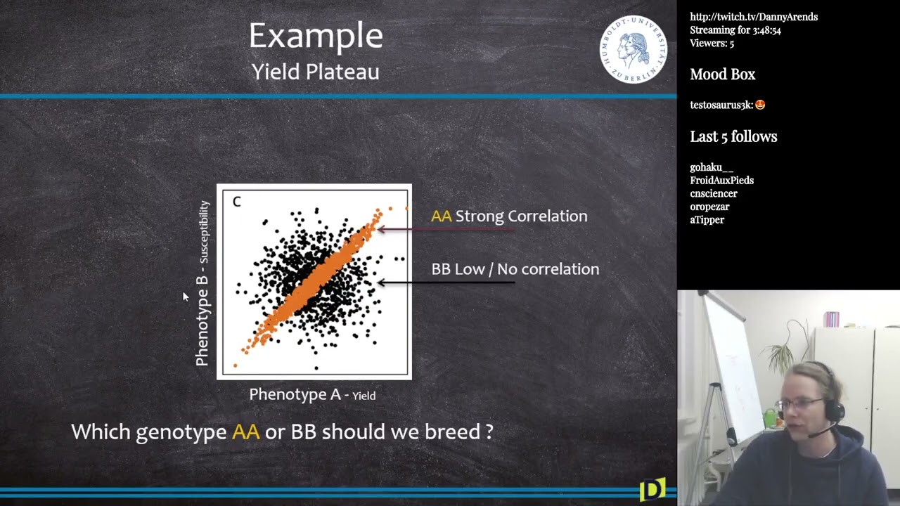
we have the aa genotypes which show
strong correlation right the same
correlation that we see overall in the
population
and we have here the bb genotype which
shows low to no correlation which you
can see that there's no like it's just a
cloud of points and there's no straight
line right so if you see a picture like
this
which genotype should we breed
should we breed the aaa individuals or
should we breed the bb individuals so
that's a question to you guys in chat if
you're still listening right so that was
the whole idea behind it right that if
you have two phenotypes which are highly
correlated overall at each marker you
look at the correlation
between the individuals which are a a
and the individuals which are bb and
then you will find if you're lucky a
locus in the genome where these two
highly correlated phenotypes are not
correlated so in this case of course if
you want to breed the next generation
you want to breed individuals which are
bb at this locus right because the bb
shows no correlation and in this case we
have a positive phenotype linked with a
negative phenotype and we can also have
like a negative phenotype length with a
negative one
and then of course you would probably
want to have the correlation and show
the lower tail
right so select the ctl genotype to
unlink two phenotypes and in the next
generation which should show a decrease
of correlation between the phenotypes
and this allows again in the next
generation to select high yield without
increasing the susceptibility
right and then in in the next generation
you would just select individuals based
on qtl information like you would
normally do
so the methodology
here i explain it using recommend name
red lines there is a package on
chrome which actually is called ctl
and this package handles many more
complex crosses so i i just explain it
here using aa and bb individuals but it
also works if you have an f2 population
where you have a a a b and b b
individuals so recombinant in red lines
um i'm
i'm
at the example here
is assuming that i have four
phenotypes which have been measured
and i have six genetic markers right so
i have four different phenotypes and six
genetic markers and um
at
every locus right at every marker there
an individual can have either a a or bb
just to simplify it for the for the
presentation
so the way that this methodology works
is first you select a phenotype called
p1 right so that's your first phenotype
then you select a genetic marker so the
first one right you split the
individuals into two groups by their
genotype so you have a group of
individuals at the fir which at the
first marker is aa and then you have a
group of individuals which at the first
marker is bb so here you have a
population for example of 100 animals
and 50 of them go into group 1 50 of
them are in group 2 because these 50 faa
these 50 fbb then what you do is you
calculate your correlation for both the
aa and the bb genotype
what you do is you do p1 times all of
the phenotype correlation vector right
so you just say well calculate the
correlation of your phenotype p1 with
the phenotypes which are showing a a
right and then you just get a vector so
phenotype one of course shows a
correlation of one to phenotype one
because two things which are equal
always have a correlation of one
p1 and p2 at this marker show 0.1 uh
correlation um
p1 and p3 0.5 p4 0.8 right so here p1
and p4 are highly correlated at this
marker
you do the same thing for the bb
individuals right so you again get a
vector with four correlation
coefficients um of course p1 versus p1
is still one um and for the other three
phenotypes you also get a correlation so
correlation in pop in the aaa
individuals correlation in the bb
individuals
so then the next step is just to
define the effect size right so the
effect size in in qtl is defined as the
difference in the mean between the aa
group and the bb group
but in in ctl mapping the ctl defect
size is calculated or defined as the
difference in correlation between the aa
and the bb groups
right just like qtl but now instead of
looking at the difference in mean we're
looking at the difference in correlation
between phenotype right and to make it
easy we're just going to take the
absolute difference right so not
negative and positive we're just going
to say that um
like
the the absolute difference right so
minus 0.1 becomes 0.1
so when we do that so here we have the
two vectors from before and now we just
calculate the difference vector so of
course p1 because the correlation in of
b1 to p1 is of course one and one the
difference is zero
the difference from p1 in aa to the
p1 to p2 and vb um is 0.1 0.2
right so we just take the difference so
we just subtract these two vectors from
each other
then the next step of course is now we
have mapped one marker
is to do all of the markers right so
what i do is i take the vector that i
just had and just put it on its side
right so now here we have the markers in
the in the columns and we have the
different phenotypes in the rows right
so this is the result from the last
slide you can check that it's
0.00.10.20.7 and indeed here you see the
same thing right and then this is the
difference vector for matrix 2 different
vector for marker 3 difference vector
for marker 4 and so on and like i told
you we assume that we only have 6.
right so i repeat this calculation for
every genetic marker so multiple
difference vector for our selected
phenotype
of course that when we map p1 against p1
it will all yield a difference of zero
right so we could have not mapped this
and just skipped it but that just for
completeness sake i just want to show
you the whole
whole matrix
let me get a sip of one
sorry it's been a long lecture
all right so here we map p1 against p1
always a zero and of course for the
other phenotypes we don't get that
so now we need to of course find what is
significant right is this difference of
0.6 in correlation is that a significant
difference so what we do is we repeat
the same thing at 10 000 times just like
i showed you guys for qtl is we break
the link between genotype and phenotype
right so in this case we're just
assigning
genotype vectors at random to the
individuals just like we did before in
qtl mapping but in qtl mapping we
assigned the phenotypes randomly
right but now since we have two
phenotypes we want an individual so the
two phenotypes of the individual to stay
the same but now we just give it a
random genotype vector in the end right
so we redo the whole analysis we
remember the maximum score and then we
make a distribution out it and then we
find our five percent and one percent
thresholds for significance values right
it's just the same way so we're just
going to permute ourselves out of
problems by just saying i'm just gonna
instead of assigning a new phenotypic
value for each individual based on the
back that we have we're now just going
to assign like a new genotype
so ctl uses 10 000 plus permutations to
add sign significant of course in the
package because i did study this stuff
for four years i also devised a method
to directly calculate your p-value using
mathematics so of course here we then
convert so we convert the differences in
correlation that we see
to probability values so how likely is
it that there is a real correlation
difference at that point and then we do
the next step which is just saying the
same as qtl where we convert the p-value
to the lot score so we just take the
minus log 10 of the p-value
so by converting this have we performed
qtl mapping for
p1 as well
so
because we we have the data anyway so we
have p1 which we can
ctl map against the four phenotypes that
we have but we can of course also just
do the qtl mapping right so for p1 we
get four vectors of lot scores from ctl
mapping right so every every
every
every correlation difference is
transformed into a lot score um
and beside that we have the information
about p1 itself right so because we can
also associate p1 with every one of the
six markers that we have
so how does this then look so this is
the way that we visualize it so we take
our qtl curve of p1 and we just plot it
on the top
and then we take the ctf curves of p1
versus the other phenotypes which we see
on the bottom
right so on the bottom is the lot score
and the negative lot score of the ctl
score and of course the on the bottom we
then see 4 or five or six or seven lines
no matter or how many phenotypes we had
all right so that was the ctl mapping
method it's a relatively easy
thing right and in the end we find loci
in the genome where we see that there's
for example a qtl controlling the
variation in p1 but we also see that at
this locus p1 loses correlation with
some of the other phenotypes
let me actually pull up one of the other
presentations that i did about ctl
mapping where we use some real data
right
just to show you guys how we can use
this information
it should be somewhere in
presentations
ctc transmission ratio distortion here
so let me open this up and
all right
can i actually easily swap that
just swap the powerpoint yes i can so
let's go to properties and then switch
to this one right
so
what we were looking at here is in
arbitropsystaliana we have metabolites
and these metabolites are known to be in
a linear pathway so we have
something called hydroxypropule which is
then using an enzyme is transformed into
material sulfoneupropyl and then using
another enzyme this is transformed into
material thiopropyl right so it's just
three metabolites with two enzymes in
the middle there is a major regulator of
this pathway on chromosome five and all
of this was known right so then i did
the ctl mapping right so the first plot
that i'm going to show you is and
remember the colors right so it's it's
green red orange right so green is on
the top of the network then green gets
transformed into red and red gets
transformed into orange
so here we see this the qtl profile of
hydroxypropyl on the top right so we see
that there's a major regulator
of
the difference in hydroxypropyl and
chromosome 5. the same thing holds for
chromosome 4 there's a marker on
chromosome 4 which also
controls the heteroxypropyl
concentration in in the plan
but then we start seeing that if we do
the ctl mapping with material sophomore
and material theoprophyl right so the
red one and the orange one we see that
we do find a little locus on chromosome
one and that is strange right because we
never had any indication from qtl
mapping that
something on chromosome one was actually
driving the hydroxypropel region but we
do get the idea that well there is
something on one which makes
which which makes hydroxypropyl lose its
regulation or
lose its correlation with the other two
phenotypes that we're looking at and we
see the same thing on chromosome 5 right
so on chromosome 5 we learn nothing new
because we already knew that there was a
major driver of this network
when we then look at the middle
phenotype in the pathway of the middle
metabolite in the pathway methyl
sulfaneopropyl
what we see is now hey that's
interesting
there is a little qtl on
chromosome 1 for the middle phenotype
so there is something on chromosome 1
which is controlling the concentration
of the the middle phenotype of course
there's also something on chromosome 5
which is kind of passed down right from
the initial one so the in the initial
concentration of hydroxypropule
is transformed into materials
sulfoneupropyl right so the more you
have at the beginning of course the more
you have from the intermediate product
as well so here we also see the um the
ctl line and we did indeed see that that
at this locus we do get the idea that
yes no there is correlation between the
amounts of sophomore of uh hydroxypropyl
sulfanium propel and the theoprovium
so when we then look at theopropyl now
we see something interesting
because if we look at the top we see
that when we do the qtl mapping of this
phenotype we don't know where the
concentration of this
this this um metabolite is controlled
from there are no significant regions
so if i would do an experiment using
material theo material theopropel
measurements right and it would scan
across the genome
i would learn that there is no locus
that is controlling the concentration of
material theopropyl
however if we look
at the ctl map we do see that we get
significant load side so we do see that
the the the method tells us there is
something on chromosome 5 which is
influencing the correlation of
theopropyl hydroxypropyl and materials
materials
sulfoneopropyl right and the same thing
again on chromosome 1.
so what we see is that
for the first two phenotypes we don't
really learn anything new except for
that there is something going on on
chromosome 1 for hydroxypropel
we learn for the middle one we don't
learn anything or not that much because
we already knew that there was something
on chromosome 5 controlling it but for
the last one we don't get any qtl and
because we get no qtl as a geneticist
you're stuck here you cannot say what's
happening to teopu
but we can from qt or from ctl mapping
we learn that no there you if you want
to influence
this phenotype you have to be on
chromosome 5 and
there might be something on chromosome 1
which can also influence it
so the idea is is that we have this
network right so this network is driven
so if we combine the qtl information
that we get so on chromosome 5 we see
that the strongest association with
chromosome 5 is with hydroxypropyl
then the the
lot score
then because this the concentration of
this one influences the concentration of
this one so we can still see the effect
of the chromosome 5 locus on this one
but we learned that this effect of
chromosome 5 is not a direct effect it
is an indirect effect it goes via
hydroxy so the thing on chromosome 5 is
not directly influencing material sulfur
neutropia it is influencing
hydroxypropel and that in turn is
influencing material sulfone protein
so the exact same thing have we then
find for this locus here we don't find
any direct association of chromosome 5
with this phenotype but based on the ctl
and the strength of the ctl right
because the thickness of the line
determines the strength we now learn and
we now start seeing that indeed this is
kind of a linear network right because
we see that the red
metabolite should be in between the two
because there is a very strong ctl from
the red one from the green one to the
red one but from the green one to the
yellow one it is much lower and from the
red one to the yellow one it's also
lower but it's still detectable right so
we can start building up this causal
network and seeing that indeed
the network should be
hydroxypropyl
causes changes in sulfoneupropyl which
then causes changes in material to
profile and without ctl mapping we would
have never looked at chromosome 5 for
this phenotype because there is no
direct association
only based on the correlation can you
see that the correlation is lost at that
point
good
so that's the whole big idea that's what
people gave me my doctor title for
seems not much but was a lot of work was
a lot of work to uh
to to do all of this and uh
thank you guys for uh actually staying
until the end
right so you can see that i actually use
the same phenotype in this presentation
as well
but
the idea is is that qtl mapping is only
a part of the puzzle qtl mapping gives
you direct effects on the means of
phenotype but in the end it's not about
single phenotypes it's about the
relationship between phenotypes and how
genetic loci kind of modify these
relationships
good so that was what i wanted to tell
you today so for today just as a quick
overview we did phenotypes heritability
i tried to explain to you guys what qtl
mapping is and how you need to use
experimental crosses i told you guys
about gwas i didn't tell you about the
bfmi it will be in the slides that i
upload but i just skipped that part
and i will talk to you i talk to you
about ctl mapping also the fine mapping
part is not directly in the in the
presentation because i skipped it today
because we were kind of running out of
time because we took an hour for the
assignments
all right so for me that's it for today
if there's any questions remarks other
things then then please let me know
throw it in the chat i think all of the
four guys that made it to the end like
you're amazing
thank you for being here
and of course for my moderator who's
also probably still here
um
bacon misha thank you guys for joining
and staying until the end
um that was it for me it's uh five so
people on youtube um see you on the flip
side
so
see you next time